Introduction
Please do not distribute. ©
THIS DOCUMENTATION IS A WORK-IN-PROGRESS, MANY CHAPTERS ARE STILL EMPTY
METROPOLIS2
METROPOLIS2 is an agent-based transport simulator.
Its main features are:
- 🚘 Mode choice (with an arbitrary number of modes, road vehicles are explicitly modeled)
- ⏱️ Continuous-time departure-time choice
- 🛣️ Deterministic route choice (for road vehicles)
- 👫 Agent based (each agent is an autonomous entity with its own characteristics and choices)
- 🚦 Modeling of road congestion (using speed-density functions and bottlenecks)
- ⏸️ Intermediary stops (with schedule preferences and stopping time at each intermediary point)
METROPOLIS2 is composed of
metrolib: a command line tool to run the transport simulations, written in Rust 🚀metropy: a command line tool to interact with METROPOLIS2’s input and output data, written in Python 🐍
What is this book?
This is the official documentation of METROPOLIS2, intended for anyone wanting to learn how to use the simulator and how it works.
It is devided in 6 chapters:
- Chapter 1: Metropy user guide
- Chapter 2: Metrolib reference
- Chapter 3: Advanced topics
- Chapter 4: Theoretical foundations
- Chapter 5: Implementation details
- Chapter 6: External tools
Metropy User Guide
Metropy is a Python command line tool to process the input / output data of the Rust simulator.
Metropy can run many operations like:
- importing a road network from OpenStreetMap data,
- generating trips from an origin-destination matrix,
- computing the walking distance of a set of trips,
- building a macroscopic fundamental graph from the results.
Requirements ☑️
- Recent Python version (3.11+).
- Git or GitHub Desktop
- QGIS with parquet support (QGIS 3.22+, GDAL 3.5+), optional (only used to visualize spatial data).
Installation 🔧
- Clone the metropy GitHub repository with the command
git clone https://github.com/Metropolis2/metropyor directly from GitHub Desktop. - Install the python packages listed in
requirements.txt. The recommended way is to install virtualenv and run the following commands from themetropydirectory:$ virtualenv env $ source venv/bin/activate $ pip install -r requirements.txt
To check that metropy has been installed correctly, you can run python -m metropy --help from the
metropy directory.
How to use 🤷♂️
Before running metropy, you need to create a TOML configuration file that will dictate how the simulation is generated (which area? what data is used to import the population? which modes are available?, etc.). All the possible parameter values in the configuration file are detailed on the Configuration page.
When your configuration is ready, simply run the command:
$ python -m metropy my-config.toml
This will run all the steps which are required to generate the simulation’s input files.
If you change some parts of the configuration and the run the command again, metropy will only execute the steps which need to be executed again (e.g., the road network is not imported again if you only changed the origin-destination matrix).
Next steps 🧭
This user guide contains a detailed description
- the Steps that metropy can run,
- the Configuration parameters,
- the Files generated.
If you prefer to learn through complete examples, have a look at Case Study 1 (detailed simulation generation with synthetic population for a small-size French city, Chambéry) or Case Study 2 (TO BE DONE).
Advanced use ⚙️
Metropy generates the simulation’s input files by executing sequentially several “Steps”, which are detailed on the Steps page. The execution order is computed automatically so that no step is executed before its prerequisite steps are executed (e.g., the walking distance is not computed before the walking network is imported).
If you don’t want to generate all input files and only require a specific step to be run, you can do
so using the optional --step argument.
For example, if you run the command:
$ python -m metropy my-config.toml --step simulation-area
metropy will only run the step osm-import and all the prerequisite steps then stop.
Getting help 🛟
Although metropy tries to be as reliable and universal as possible, various issues can arise when running metropy due to the complexity of the process involved and the variety of datasets around the world. Many error messages have been included in the library to explain as clearly the issues that might have occurred.
If you found a bug or if there is a problem that you cannot fix, feel free to open an issue on the GitHub repository.
Steps
Table of Contents
Step simulation-area
- Description: The
simulation-areastep creates a polygon of the simulation area in which all trips take place. The polygon is used, for example, to filter out roads outside the simulation area. - Requirements: Optional (default is to not filter by any area).
- Prerequisite: None
- Output file(s): Simulation area
- Estimated running time: A few seconds (except for large OpenStreetMap imports).
There are 4 different ways to generate the polygon, described below.
Method 1: Providing a bounding box
The easiest way to specify the simulation area is to define its bounding box. This however means that the area is limited to rectangles.
The bounding box needs to be specified as the bbox value, which expects a list of coordinates
[minx, miny, maxx, maxy].
By default, the coordinates need to be specified in the simulation CRS.
If you want to specify them in WGS84 (longitude, latitude), you can use bbox_wgs = true.
You can go to www.openstreetmap.org to identify the bounding box of a region (as WGS84 coordinates), using the “Export” button.
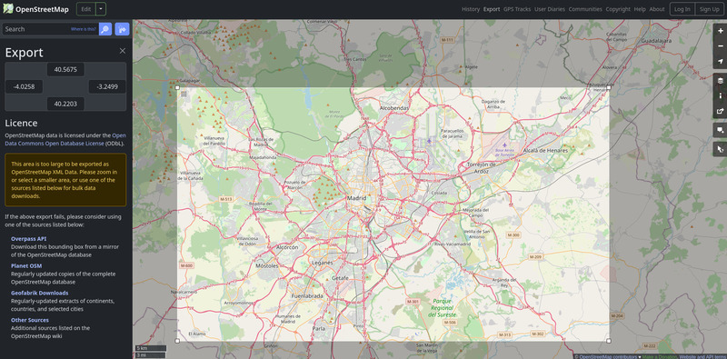
[simulation_area]
bbox = [1.4777, 48.3955, 3.6200, 49.2032]
bbox_wgs = true
Method 2: Providing a geospatial file with polygon(s)
If you already have a set of polygons which jointly form the entire area (e.g., the administrative boundaries of all municipalities to be considered), you can simply provide as input a geospatial file with those polygons. Then, metropy will read the file and define the polygon of the simulation area as the union of all polygons. If there is a single polygon (e.g., the administrative boundary of the region to be considered), metropy will simply use it as the simulation area polygon.
The file can use any GIS format that can be read by geopandas (e.g., Parquet, Shapefile, GeoJson).
It needs to be specified as the polygon_file value.
[simulation_area]
polygon_file = "path/to/polygon/filename"
Method 3: Reading a French metropolitan area
A French metropolitan area (aire d’attraction d’une ville) is a type of statistical area defined by the French national statistics office INSEE. It is defined by considering the commuting patterns between cities, making it well adapted to define areas for transport simulations.

The database for these aires d’attraction des villes is publicly available on the
INSEE website.
Metropy can automatically download the database and read the polygon of an area if you set the
aav_name parameter to one of the existing area.
The areas’ name is usually the name of the biggest city in the area.
[simulation_area]
aav_name = "Paris"
If the automatic download does not work, you can download the file locally and tell metropy to use that version:
- Go to the INSEE page of the aires d’attraction des villes database: https://www.insee.fr/fr/information/4803954
- Download the zip file “Fonds de cartes des aires d’attraction des villes 2020 au 1er janvier 2024”
- Unzip the file. You will get two zip files representing shapefiles:
aav2020_2024.zip(polygons of the areas) andcom_aav2020_2024.zip(polygons of the municipalities). Only the former is needed. - In the section
[simulation_area]of the configuration, add the linesaav_filename = "path/to/aav2020_2024.zip"andaav_name = "YOUR_AAV_NAME".
[simulation_area]
aav_name = "Paris"
aav_filename = "path/to/aav2020_2024.zip"
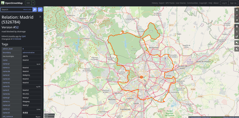
Method 4: Reading OpenStreetMap’s administrative boundaries
Administrative boundaries of various subdivisions are specified directly on OpenStreetMap (e.g.,
states, counties, municipalities), with the tags
admin_level=* and
boundary=administrative.
The OpenStreetMap wiki has a
table
indicating the meaning of each admin_level value by country.
For example, admin_level=6 represents counties in the U.S. and départements in France.
You can use metropy to create the simulation area by reading one or more administrative
boundaries from OpenStreetMap data.
First, you need to set the osm_file value to the path to the OpenStreetMap file.
In the [simulation_area] section, the osm_admin_level value represents the admin_level value
to be used as filter and the osm_name value is a list of the subdivisions names to be selected.
For example, to get the polygon of Madrid, you can use:
osm_file = "path/to/spain.osm.pbf"

[simulation_area]
osm_admin_level = 8
osm_name = ["Madrid"]
Or, to get the polygon of Paris and the surrounding departments, you can use:
osm_file = "path/to/france.osm.pbf"

[simulation_area]
osm_admin_level = 6
osm_name = ["Paris", "Hauts-de-Seine", "Seine-Saint-Denis", "Val-de-Marne"]
Buffering the simulation area’s polygon
Regardless of the method used, the buffer parameter allows you to extend (or shrink) the polygon
of the simulation area by a given amount, expressed in the unit measure of the CRS (usually meters).
Use positive values to extend the area, and negative values to shrink it.
[simulation_area]
polygon_file = "path/to/polygon/filename"
buffer = 500
Step osm-road-import
- Description: Extract the road network, as a graph of directed edges, from OpenStreetMap data.
- Requirements: Required.
- Prerequisite:
simulation-area(optional) - Output file(s): Raw edges, Urban areas (if
urban_landuseis set) - Estimated running time: TODO
# Example configuration.
[osm_road_import]
highways = [
  "motorway",
  "motorway_link",
  "trunk",
  "trunk_link",
  "primary",
  "primary_link",
  "secondary",
  "secondary_link",
  "tertiary",
  "tertiary_link",
  "living_street",
  "unclassified",
  "residential",
]
urban_landuse = [
  "commercial",
  "construction",
  "education",
  "industrial",
  "residential",
  "retail",
]
urban_buffer = 50
With this step, metropy will read the OpenStreetMap data from osm_file and will select all the
ways which satisfy all the following criteria:
- The way has a
highwaytag whose value is in thehighwaysconfiguration parameter. - The way does not have a
accesstag or theaccessvalue is equal toyes,permissiveordestination. - The way’s geometry intersects with the simulation area polygon (if any).
For each valid way, metropy will read the following tags (when they are specified): name (or
addr:street, or ref as fallback), toll, junction (to detect roundabouts), oneway,
maxspeed (or maxspeed:forward and maxspeed:backward), lanes (or lanes:forward and
lanes:backward).
In addition, metropy will flag the ways with traffic signals, give-way signs and stop signs by
reading the highway tag of the ways’ nodes.
From the extracted ways and their data, metropy will then create the edges of the road network graph with the following operations:
- Bidirectional ways (
oneway=no) are split in two directed edges. - Ways are divided in multiple edges when a node of the way that is neither the first nor the last node is an intersection (i.e., another way is intersecting the middle of this way).
Urban areas
If the urban_landuse configuration parameter is defined, then
metropy will also read all the areas from the OpenStreetMap data to retrieve those matching the
following criteria.
- The area has a
landusetag whose value in in theurban_landusevalues, - The area’s geometry intersects the simulation area polygon (if any).
The geometries of the valid areas will then be buffered based on the urban_buffer configuration
parameter and the edges whose geometry is fully contains within urban areas will be flagged as
urban.
The urban areas are saved to the Urban areas file.
Additional output
Metropy will output some statistics regarding the operations performed in the file
osm-road-import/output.txt and it will generate some graphs in the directory
graphs/osm-road-import/.
Configuration
TODO: link to the steps in the requirements.
This page describes all the key/value pairs that can be specified in the TOML configuration file.
It is recommended to have some basic knowledge on the TOML syntax, for example by reading this page.
Table of Contents
Notes
- Path strings: It is recommended to use slash
/instead of backslash\as directory separator. The path can be absolute or relative to the working directory (i.e., the directory from which metropy is run). - Geospatial file: Either a
.parquetfile with ageometrycolumn or any file that can be read withgeopandas.read_file(e.g., shapefile, geopackage, GeoJson).
Complete exemple
TODO
Main variables
main_directory
- Description: Directory where the files generated by metropy will be stored.
- Allowed values: String representing a valid path.
- Requirements: Required for all steps.
- Example:
"paris/output/" - Note: If the directory does not exist, it will be created automatically by metropy.
crs
- Description: Projected coordinate system to be used for spatial operations.
- Allowed values: Any value accepted by
pyproj.CRS.from_user_input() - Requirements: Required for all steps involving spatial operations.
- Example:
"EPSG:2154"(Lambert projection for France) - Note: You can use the epsg.io website to find a projected coordinate system that is adapted for your study area. It is strongly recommended that the unit of measure is meter. If you use a coordinate system for an area of use that is not adapted or with an incorrect unit of measure, then some operations might fail or the results might be erroneous (like road length being overestimated).
osm_file
- Description: Path to the OpenStreetMap file (
.osmor.osm.pbf) with data for the simulation area. - Allowed values: String representing a valid path to a
.osmor.osm.pbffilename. - Requirements: Conditionally required for steps
simulation-area,osm-road-importandosm-walk-import. - Example:
"data/osm/france-250101.osm.pbf" - Note: You can download extract of OpenStreetMap data for any region in the world through the Geofabrik website. You can also download data directly from the OSM website, using the “Export” button, although it is limited to small areas.
[simulation_area] table
bbox
- Description: Bounding box to be used as simulation area.
- Allowed values: List of 4 floats.
- Requirements: Conditionally required for step
simulation-area. - Example:
[1.4777, 48.3955, 3.6200, 49.2032] - Note: The values need to be specified as
[minx, miny, maxx, maxy], in the simulation’s CRS. Ifbbox_wgs = true, the values need to be specified in WGS 84 (longitude, latitude).
bbox_wgs
- Description: Whether the
bboxvalues are specified in the simulation CRS (false) or in WGS84 (true). - Allowed values: Boolean.
- Requirements: Optional for step
simulation-area(default isfalse). - Example:
true
polygon_file
- Description: Path to the geospatial file containing polygon(s) of the simulation area.
- Allowed values: String representing a valid path to a geospatial file.
- Requirements: Conditionally required for step
simulation-area. - Example:
"data/my_area.geojson"
aav_name
- Description: Name of the Aire d’attraction des villes to be selected.
- Allowed values: String of a value that appears in the column
libaav2024of theaav_filenamefile. - Requirements: Conditionally required for step
simulation-area. - Example:
"Paris"
aav_filename
- Description: Path to the shapefile of the French’s Aires d’attraction des villes.
- Allowed values: String representing a valid path to the
.zipfile or.shpfile from INSEE (with columnlibaav20xx). - Requirements: Optional for step
simulation-area. - Example:
"data/aav2020_2024.zip" - Notes: When
aav_filenameis not specified butaav_nameis set, metropy will attempt to automatically download the shapefile.
osm_admin_level
- Description: Administrative level to be considered when reading administrative boundaries.
- Allowed values: Integer.
- Requirements: Conditionally required for step
simulation-area. - Example:
6 - Notes: See this page for a table with the meaning of all possible value for each country.
osm_name
- Description: List of subdivision names to be considered when reading administrative boundaries.
- Allowed values: List of strings.
- Requirements: Conditionally required for step
simulation-area. - Example:
["Madrid"] - Notes: The values are compared with the
name=*tag of the OpenStreetMap features. Be careful, the name can sometimes be in the local language.
buffer
- Description: Distance by which the polygon of the simulation area must be extended or shrinked.
- Allowed values: Number.
- Requirements: Optional for step
simulation-area(default is 0). - Example:
500 - Notes: The value is expressed in the unit of measure of the CRS (usually meter). Positive values extend the area, while negative values shrink it.
[osm_road_import] table
highways
- Description: List of
highway=*OpenStreetMap tags to be considered as valid road ways. - Allowed values: List of strings.
- Requirements: Required for step
osm-road-import. - Example:
["motorway", "motorway_link", "trunk", "trunk_link", "primary", "primary_link"] - Notes: For a list of
highwaytags with description, see the OpenStreetMap wiki.
urban_landuse
- Description: List of
landuse=*OpenStreetMap tags that define an urban area. - Allowed values: List of strings.
- Requirements: Optional for step
osm-road-import(default is to consider all the area as being rural). - Example:
["residential", "industrial", "commercial", "retail"] - Notes: For a list of
landusetags with description, see the OpenStreetMap wiki. The urban areas are used to defined an urban vs rural flag on roads, which is in turn used to define default values (e.g., default speed limit of 50 km/h on urban roads vs 80 km/h on rural roads).
urban_buffer
- Description: Distance by which the polygons of the urban areas will be buffered.
- Allowed values: Number.
- Requirements: Optional for step
osm-road-import(default is 0). - Example:
50 - Notes: The value is expressed in the unit of measure of the CRS (usually meter). Positive values extend the area, while negative values shrink it. A road edge must be entirely contained within urban areas to be classified as a urban edge so it is recommended to use a positive value to correctly identify urban edges.
Files
Table of Contents
output/
├── graphs
│   └── road_network.osm
│       ├── lanes_distribution_length_weights.pdf
│       ├── lanes_distribution.pdf
│       ├── length_distribution.pdf
│       ├── road_type_pie_length_weights.pdf
│       ├── road_type_pie.pdf
│       ├── speed_limit_distribution_length_weights.pdf
│       └── speed_limit_distribution.pdf
├── maps
│   ├── chambery_aav.jpg
│   └── france_aav.jpg
├── osm-road-import
│   ├── edges_raw.parquet
│   ├── osm_output.txt
│   └── urban_areas.parquet
└── simulation_area.parquet
Files outside of directories
Simulation area
- Filename:
simulation_area.parquet - Geospatial: Yes
- Columns:
geometry: Polygon of the simulation area
- Comment: The file contains only a single feature, representing the simulation area.
Directory osm-road-import
Raw edges
- Filename:
edges_raw.parquet - Geospatial: Yes
- Columns:
geometry: LineString of the edgeedge_id(UInt64): Identifier of the edgeosm_id(UInt64): Identifier of the corresponding OpenStreetMap waysource(UInt64): Identifier of the OpenStreetMap node of the edge’s first nodetarget(UInt64): Identifier of the OpenStreetMap node of the edge’s last noderoad_type(String): Value of thehighwaytagname(String): Value of thenametag (oraddr:street, orrefas fallbacks)toll(Boolean): Whether the way has tagtoll=yesroundabout(Boolean): Whether the way has tagjunction=roundaboutoneway(Boolean): Whether the way has tagoneway=yesspeedlimit(Float64): Speed limit on the edge, in km/h (if available)lanes(Float64): Number of lanes on the edge (if available)give_way(Boolean): Whether the edge ends with a give-way signstop(Boolean): Whether the edge ends with a stop signtraffic_signals(Boolean): Whether the edge ends with traffic signalslength(Float64): Length of the edge’s geometry, in the same unit as the CRSurban(Boolean): Whether the edge is within urban areas
Urban areas
- Filename:
urban_areas.parquet - Geospatial: Yes
- Columns:
geometry: LineString of the edgeosm_id(UInt64): Identifier of the corresponding OpenStreetMap way (even numbers) or relation (odd numbers), see https://docs.osmcode.org/pyosmium/latest/user_manual/03-Working-with-Geometries/#the-pyosmium-area-typelanduse(String): Value of thelandusetag
Case Study 1: Chambéry
Table of Contents
Chambéry
Chambéry is a French city in the Savoie department, near the Alps. In 2021, the population of Chambéry was 59,856.
.JPG)
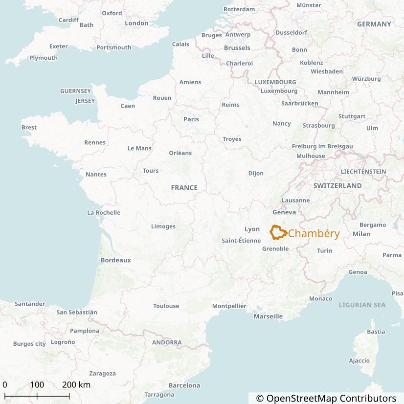
It is the largest city of the Chambéry Metropolitan area (Aire d’attraction de Chambéry) which has a population of 261,463 and an area of 1,147 km² (2021). The Metropolitan area of Chambéry consists of 115 French municipalities.
Chambéry has been selected for this case study due to its small size (reducing running times) and the availability of a recent travel survey (2022).
General Configuration
Before running the metropy pipeline, we need to create the TOML configuration file that specifies all the parameters of the simulation.
Create the config-chambery.toml file with the following content:
# File: config-chambery.toml
main_directory = "./chambery/output/"
crs = "EPSG:2154"
osm_file = "./chambery/data/rhone-alpes-250101.osm.pbf"
The main_directory variable represents the directory in which all the output files generated by
the pipeline will be saved.
The directory will be created automatically if it does not exist yet.
The crs variable represents the projected coordinate system to be used for all operations with
the spatial data (such as measuring the length of the road links).
The value "EPSG:2154" represents the Lambert-93 projection, which is
adapted for any area in Metropolitan France.
The osm_file variable specifies the path to the OpenStreetMap input file that will be used to
import the road and walking network.
We use the extract of the Rhône-Alpes French administrative region from 2025-01-01, that can be
downloaded from Geofabrik (click on
raw directory index to access older versions).
The Rhône-Alpes region is adapted for our case study given that the Chambéry urban area is full
contained within it.
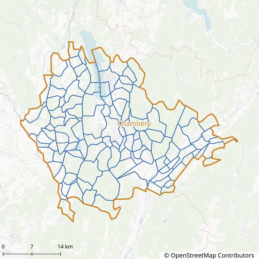
Simulation Area
- Step:
simulation-area - Running time: 2 seconds
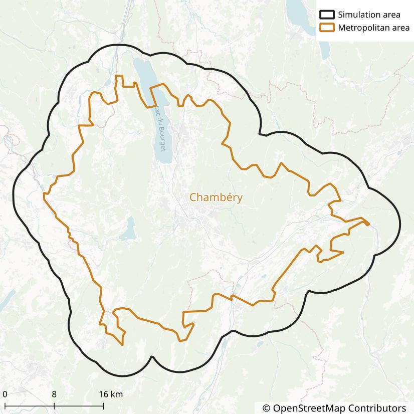
We define the simulation area as the Chambéry Metropolitan area (aire d’attraction) so that we get an area large enough to encompass most of the trips from and to Chambéry’s municipality.
To tell metropy to create the simulation area from the Chambéry Metropolitan area, add the following section to the configuration:
[simulation_area]
aav_name = "Chambéry"
buffer = 8000
The buffer = 8000 line tells metropy to extend the area by 8 kilometers in all directions.
This is used to include roads in the simulation that are not inside the Metropolitan area but that
could be taken when traveling between two municipalities within the area.
The output file ./chambery/output/simulation_area.parquet can be opened with QGIS to draw a map.
OpenStreetMap Road Import
- Step:
osm-road-import - Running time: 2 minutes
We use the osm-road-import step to import the road network from OpenStreetMap.
The step will read the osm_file variable previously defined.
Add the following section to the configuration:
[osm_road_import]
highways = [
  "motorway",
  "motorway_link",
  "trunk",
  "trunk_link",
  "primary",
  "primary_link",
  "secondary",
  "secondary_link",
  "tertiary",
  "tertiary_link",
  "living_street",
  "unclassified",
  "residential",
]
urban_landuse = [
  "commercial",
  "construction",
  "education",
  "industrial",
  "residential",
  "retail",
  "village_green",
  "recreation_ground",
  "garages",
  "religious",
]
urban_buffer = 50
The highways parameter lists all the OSM
highway tags to be imported.
In this case, all the standard tags are considered, including living streets, residential streets
and unclassified streets.
We do not consider however the service and road tags, which usually represent car park alleys or
other special roads we are not interested in.
The urban_landuse parameter lists all the OSM
landuse tags to be classified as urban.
The roads which are fully contained within urban areas will be classified as “urban”.
The urban areas are extended by 50 meters, through the urban_buffer parameter, so that roads
partially outside urban areas are also classified as “urban”.
After the step is completed, some statistics are reported in the file
./chambery/output/osm-road-import/output.txt.
They show that the imported road network has:
- 37 088 nodes
- 77 884 edges
- The total length of edges is 13 990 km
- 69.4 % of edges are classified as “urban”
- 2.2 % of edges are roundabouts
- 0.5 % of edges have traffic signals
- 1.0 % of edges have a stop sign
- 1.3 % of edges have a give-way sign
- 1.0 % of edges have tolls
- 68.7 % of edges do not have a speed limit reported
- 84.4 % of edges do not have a number of lanes reported
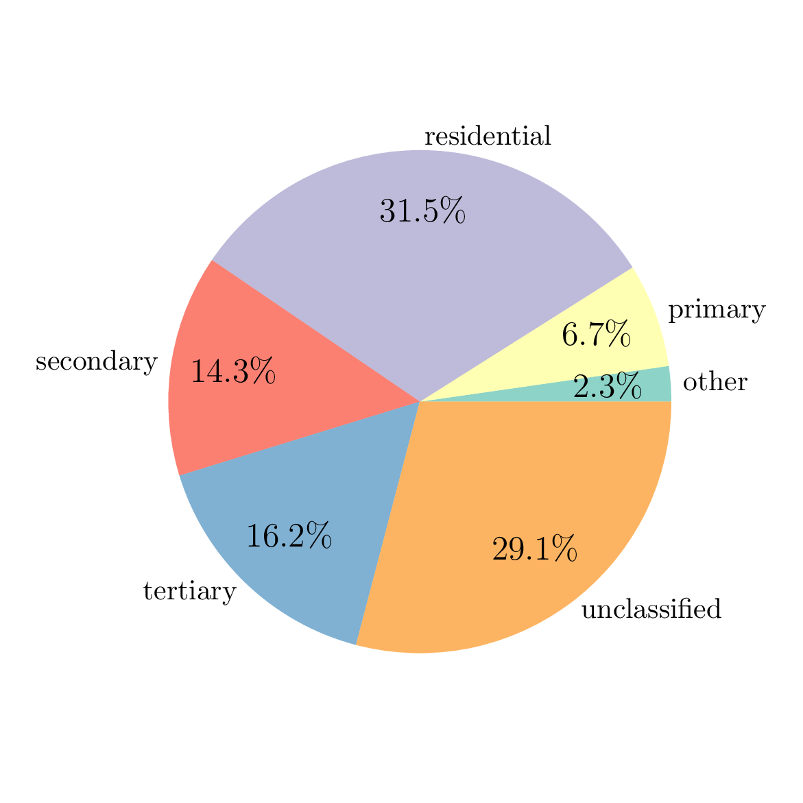
The directory ./chambery/output/graphs/osm-road-import/ also contains some graphs generated from
the imported data.
For example, the following pie chart reports the share of edges by road type (the category “other”
regroup all road types with few observations).
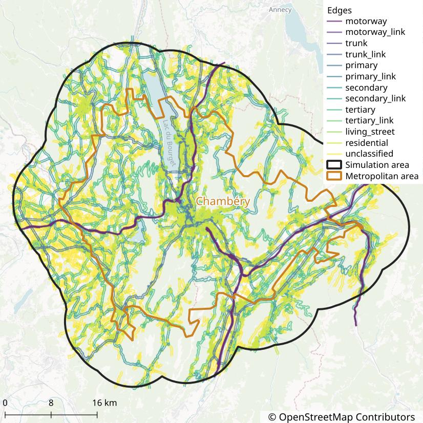
The two output files ./chambery/output/osm-road-import/edges_raw.parquet and
./chambery/output/osm-road-import/urban_areas.parquet can be opened with QGIS to draw a map of
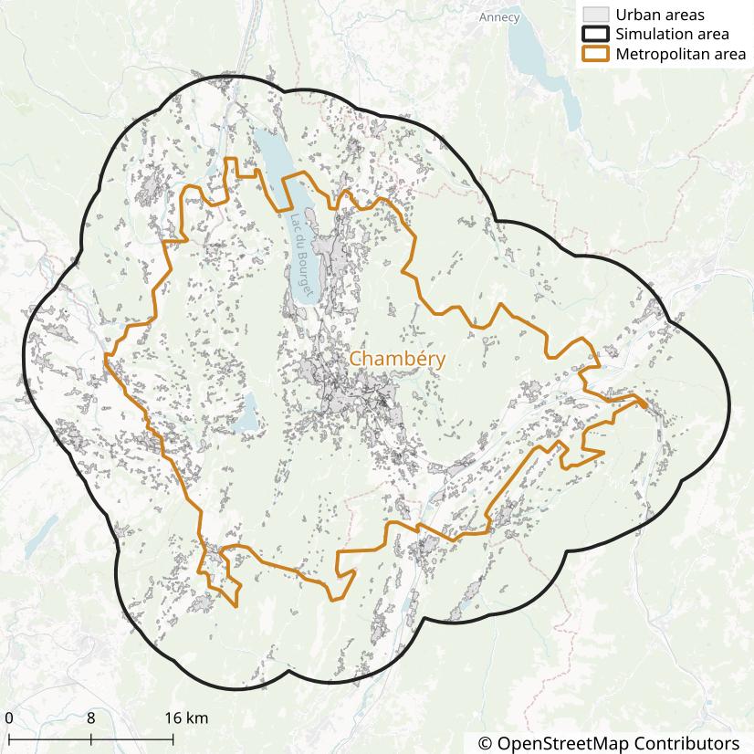
edges…
and urban areas…
Getting Started
This chapter of the book teaches how to write and understand the input files, how to run the simulator and how to read and understand the output files. It is intended for the users that want to run small- or large-scale simulations with METROPOLIS2. It can be read in any order. The users should not be afraid to skip some sections and come back to them when needed.
Glossary
- Agent: Autonomous entity choosing and performing one (and only one) travel alternative for each simulated day.
- Alternative: See travel alternative.
- Car: Denote a commonly used vehicle type, or a specific vehicle instance of this vehicle type.
- Destination: Ending node of a trip.
- Edge: Segment of the road-network graph representing a road.
- Intersection: Point where multiple roads cross / intersect. Represented by a node on the road-network graph.
- Link: See road or edge.
- Mode: Mean / manner of performing a trip (e.g., car, public transit, walking).
- Node: Point at the intersection of multiple edges on the road-network graph.
- Origin: Starting node of a trip.
- Road: Segment of the road network that is used by vehicles to move around.
- Road network: Infrastructures that can be used by vehicles to perform road trips. It is defined as a graph of nodes and edges.
- Road trip: Trip to go from an origin to a destination using a vehicle traveling on the road network.
- Route: Sequence of edges, or equivalently roads, representing the trip made by a vehicle on the road network to connect an origin to a destination.
- Travel alternative: Sequence of trips to be performed by an agent. The sequence can be empty if the agent is not traveling.
- Trip: Act of traveling from one place to another. See road trip and virtual trip.
- Vehicle: Object, such as a car, that can move / travel on a road network.
- Vehicle type: Definition of the characteristics shared by multiple vehicles.
- Virtual trip: Trip with an exogenous travel time (i.e., a travel time independent from the choices of the other agents).
Input
The main input file of METROPOLIS2 is a JSON file defining the parameters of the simulation. This file gives the path to the other input files to be read by METROPOLIS2. These input files can be in either Parquet or CSV format and they are divided two categories:
- Population input: the collection of agents, with their travel alternatives to simulate.
- Road network: the definition of the infrastructure that can be used by road vehicles.
Parameters
Table of Contents
The parameters of a METROPOLIS2’s simulation are defined in a JSON file.
Examples
Minimal working example:
{
  "input_files": {
    "agents": "input/agents.parquet",
    "alternatives": "input/alternatives.parquet"
  },
  "period": [21600.0, 43200.0]
}
Complete example:
{
  "input_files": {
    "agents": "input/agents.parquet",
    "alternatives": "input/alts.parquet",
    "trips": "input/trips.parquet",
    "edges": "input/edges.parquet",
    "vehicle_types": "input/vehicles.parquet",
    "road_network_conditions": "input/edge_ttfs.parquet"
  },
  "output_directory": "output/",
  "period": [0.0, 86400.0],
  "road_network": {
      "recording_interval": 50.0,
      "approximation_bound": 1.0,
      "spillback": true,
      "backward_wave_speed": 4.0,
      "max_pending_duration": 20.0,
      "constrain_inflow": true,
      "algorithm_type": "Best"
  },
  "learning_model": {
    "type": "Exponential",
    "value": 0.01
  },
  "init_iteration_counter": 1,
  "max_iterations": 2,
  "update_ratio": 1.0,
  "random_seed": 19960813,
  "nb_threads": 8,
  "saving_format": "Parquet",
  "only_compute_decisions": false
}
Format
The following table describes all the possible key-value pairs in the parameters JSON file.
| Key | Value data type | Conditions | Constraints | Description |
|---|---|---|---|---|
input_files | InputFiles | Mandatory | See below | |
output_directory | Path | Optional | Directory where the output files of METROPOLIS2 will be stored. If omitted, the current working directory is used. If the given directory does not exist, it is created. | |
period | Array of two Floats | Mandatory | Length of the interval is positive | Time interval defining the domain of the travel-time functions. Also the departure-time period of the agents when the dt_choice.period parameter is omitted. |
init_iteration_counter | Integer | Optional | Positive number | Initial iteration counter of the simulation. The iteration counter is only used in the output and in the function of some learning models. Default is 1. |
max_iterations | Integer | Optional | Positive number | Maximum number of iterations to run. Deault is to run a single iteration. |
road_network | RoadNetworkParameters | Optional | See below | |
learning_model | LearningModel | Optional | See below | |
update_ratio | Float | Optional | Between 0.0 and 1.0 | Share of agents (selected at random) that can update their choices at each iteration. Default is to allow all agents to update their choices at each iteration. |
random_seed | Integer | Optional | Non-negative number | Random seed used for METROPOLIS2’s random number generator. The only randomness in METROPOLIS2 is due to the update_ratio parameter. Default is to use entropy to generate a seed. |
nb_threads | Integer | Optional | Non-negative number | Number of threads used for parallel computing. If nb_threads is 0, all the available threads are used. Default value is 0. |
saving_format | String | Optional | Possible values: "Parquet", "CSV" | Format used for METROPOLIS2’s output files. Default is to use Parquet. |
only_compute_decisions | Boolean | Optional | If true, METROPOLIS2 only runs the demand model once then stops, returing the travel decisions of the agents. Default is false. |
Path
The input files and output directory of the simulation are defined in the parameters JSON file as paths.
Each path is a string representing either a relative path or an absolute path. The relative paths are interpreted as being relative to the directory where the parameters file is located. In case of issues when working with relative paths, try with absolute paths.
We recommend using slash / instead of backslash \ in the paths.
InputFiles
The value corresponding to the key input_files must be a JSON Object with the following key-value
pairs.
| Key | Value data type | Conditions | Constraints | Description |
|---|---|---|---|---|
agents | Path | Mandatory | Path to the input Parquet or CSV file with the agents to simulate. | |
alternatives | Path | Mandatory | Path to the input Parquet or CSV file with the alternatives of the agents. | |
trips | Path | Optional | Path to the input Parquet or CSV file with the trips of the alternatives. If omitted, no trip is simulated (the alternatives are no-trip alternatives). | |
edges | Path | Optional | Path to the input Parquet or CSV file with the edges composing the road network. If omitted, there is no road network (not possible if there are some road trips). | |
vehicle_types | Path | Optional | Path to the input Parquet or CSV file with the vehicle types. The path can be omitted if and only if there is no (i.e., edges and vehicle_types are either both valid or both empty). | |
road_network_conditions | Path | Optional | Path to the input Parquet or CSV file with the edges’ travel-time functions, to be used as starting network conditions. If omitted, the starting network conditions are assumed to be the free-flow conditions. |
LearningModel
Let \( \hat{T}_{\kappa} \) be the expected travel-time function for iteration \( \kappa \) and let \( T_{\kappa} \) be the simulated travel-time function at iteration \( \kappa \).
METROPOLIS2 supports the following learning models.
Linear learning model
\[ \hat{T}_{\kappa+1} = \frac{1}{\kappa + 1} T_{\kappa} + \frac{\kappa}{\kappa + 1} \hat{T}_{\kappa}, \] such that, by recurrence, \[ \hat{T}_{\kappa+1} = \frac{1}{\kappa} \sum_{i=0}^{\kappa} T_{\kappa}. \]
JSON representation:
{
  [...]
  "learning_model": {
    "type": "Linear"
  }
  [...]
}
Exponential learning model
\[ \hat{T}_{\kappa+1} = \frac{\lambda}{a_{\kappa+1}} T_{\kappa} + (1 - \lambda) \frac{a_{\kappa}}{a_{\kappa+1}} \hat{T}_{\kappa}, \] with \[ a_{\kappa} = 1 - (1 - \lambda)^{\kappa}, \] such that, by recurrence, \[ \hat{T}_{\kappa+1} = \frac{1}{a_{\kappa}} \lambda \sum_{i=0}^{\kappa} (1 - \lambda)^i T_{\kappa}. \]
The parameter \( \lambda \) is called the smoothing factor. With \( \lambda = 0 \), the exponential learning model is equivalent to a linear learning model (see above). With \( \lambda = 1 \), the predicted values for the next iteration are equal to the simulated values, i.e., \( \hat{T}_{\kappa+1} = T_{\kappa} \).
The parameter \( \lambda \) must be between 0 and 1.
JSON representation (where “value” corresponds to the \( \lambda \) parameter):
{
  [...]
  "learning_model": {
    "type": "Exponential",
    "value": 0.05
  }
  [...]
}
Unadjusted Exponential learning model
\[ \hat{T}_{\kappa+1} = \lambda T_{\kappa} + (1 - \lambda) \hat{T}_{\kappa}. \]
The parameter \( \lambda \) must be between 0 and 1.
JSON representation (where “value” corresponds to the \( \lambda \) parameter):
{
  [...]
  "learning_model": {
    "type": "ExponentialUnadjusted",
    "value": 0.05
  }
  [...]
}
Quadratic learning model
\[ \hat{T}_{\kappa+1} = \frac{\sqrt{\kappa}}{\sqrt{\kappa} + 1} T_{\kappa} + \frac{1}{\sqrt{\kappa} + 1} \hat{T}_{\kappa}. \]
JSON representation:
{
  [...]
  "learning_model": {
    "type": "Quadratic"
  }
  [...]
}
Genetic learning model
\[ \hat{T}_{\kappa+1} = \big(T_{\kappa} \cdot \hat{T}_{\kappa}^{\kappa}\big)^{1 / (\kappa + 1)}. \]
JSON representation:
{
  [...]
  "learning_model": {
    "type": "Genetic"
  }
  [...]
}
RoadNetworkParameters
The RoadNetworkParameters value is an Object with the following key-value pairs:
| Key | Value data type | Conditions | Constraints | Description |
|---|---|---|---|---|
recording_interval | Float | Mandatory | Positive number | Time interval, in seconds, between two breakpoints in the expected and simulated network conditions (the edge-level travel-time functions). |
approximation_bound | Float | Optional | Non-negative number | When the difference between the minimum and the maximum value of a travel-time function is smaller than this bound, in seconds, the travel-time function is assumed to be constant. Default value is zero, i.e., there is no approximation. |
spillback | Boolean | Optional | If true, the number of vehicles on a road is limited by the total road length. Default is true. | |
backward_wave_speed | Float | Optional | Positive number | The speed, in meters per second, at which the holes created by a vehicle leaving a road is propagating backward (so that a pending vehicle can enter the road). By default, the holes propagate backward instantaneously. |
max_pending_duration | Float | Mandatory if spillback is true, ignored otherwise | Positive number | Maximum amount of time, in seconds, that a vehicle can spend waiting to enter the next road. |
constrain_inflow | Boolean | Optional | If true, the bottlenecks limit the entry and exit flows of the road. If false, only the exit flow is limited (this is the behavior in MATSim). Default is true. | |
algorithm_type | String | Optional | Possible values: "Best", "Intersect", "TCH" | Algorithm type to use when computing the origin-destination travel-time functions. "Intersect" is recommended when the number of unique origins and destinations represent a relatively small part of the total number of nodes in the graph, but it consumes more memory. Default is "Best" (METROPOLIS2 tries to guess the fastest algorithm). |
Agents
Table of Contents
CSV / Parquet representation
In METROPOLIS2, agents can choose between various travel alternatives, where each travel alternative is composed of one or more trips. Following this hierarchy, the population input is divided in three files:
agents.parquet(oragents.csv)alts.parquet(oralts.csv)trips.parquet(ortrips.csv)
Agents
| Column | Data type | Conditions | Constraints | Description |
|---|---|---|---|---|
agent_id | Integer | Mandatory | No duplicate value, no negative value | Identifier of the agent (used to match with the alternatives and used in the output) |
alt_choice.type | String | Optional | Possible values: "Logit", "Deterministic" | Type of choice model for the choice of an alternative (See Discrete choice model). If null, the agent always chooses the first alternative. |
alt_choice.u | Float | Mandatory if alt_choice.type is "Logit", optional if alt_choice.type is "Deterministic", ignored otherwise | Between 0.0 and 1.0 | Standard uniform draw to simulate the chosen alternative using inverse transform sampling. For a deterministic choice, it is only used in case of tie and the default value is 0.0 (i.e., the first value is chosen in case of tie). |
alt_choice.mu | Float | Mandatory if alt_choice.type is "Logit", ignored otherwise | Positive number | Variance of the stochastic terms in the utility function, larger values correspond to “more stochasticity” |
alt_choice.constants | List of Float | Optional if alt_choice.type is "Deterministic", ignored otherwise | Constant value added to the utility of each alternative. Useful to simulate a Multinomial Logit model (or any other discrete-choice model) with randomly drawn values for the stochastic terms. If the number of constants does not match the number of alternatives, the constants are cycled over. |
Alternatives
| Column | Data type | Conditions | Constraints | Description |
|---|---|---|---|---|
agent_id | Integer | Mandatory | Value must exist in the agents file | Identifier of the agent |
alt_id | Integer | Mandatory | No duplicate value over agents, no negative value | Identifier of the agent’s alternative (used to match with the trips and used in the output) |
origin_delay | Float | Optional | Non-negative number | Time in seconds that the agent has to wait between the chosen departure time and the start of the first trip. Default is zero. |
dt_choice.type | String | Mandatory if the alternative has at least one trip, ignored otherwise | Possible values: "Constant", "Discrete", "Continuous" | Type of choice model for the departure-time choice (See Departure-time choice). |
dt_choice.departure_time | Float | Mandatory if dt_choice.type is "Constant", ignored otherwise | Non-negative number | Departure time that will always be selected for this alternative |
dt_choice.period | List of Float | Optional if dt_choice.type is "Discrete" or "Continuous", ignored otherwise | The list must have exactly two values, both values must be positive, the second value must be larger than the first one, the period must be within the simulation period | Period of time [t0, t1] in which the departure time is chosen, where t0 and t1 are expressed in number of seconds after midnight. Only relevant for "Discrete" and "Continuous" departure-time model. If null, the departure time is chosen over the entire simulation period. |
dt_choice.interval | Float | Mandatory if dt_choice.type is "Discrete", ignored otherwise | Positive number | Time in seconds between two intervals of departure time. |
dt_choice.offset | Float | Optional if dt_choice.type is "Discrete", ignored otherwise | Offset time (in seconds) added to the selected departure time. If it is zero (default), the selected departure times are always the center of the choice intervals. It is recommanded to set this value to a random uniform number in the interval [-interval / 2, interval / 2] so that the departure times are spread uniformly instead an interval. | |
dt_choice.model.type | String | Mandatory if dt_choice.type is "Discrete" or "Continuous", ignored otherwise | Possible values: "Logit", "Deterministic" (only for "Discrete") | Type of choice model for departure-time choice. |
dt_choice.model.u | Float | Mandatory if dt_choice.type is "Discrete" or "Continuous", ignored otherwise | Between 0.0 and 1.0 | Standard uniform draw to simulate the chosen alternative using inverse transform sampling. For a deterministic choice, it is only used in case of tie. |
dt_choice.model.mu | Float | Mandatory if dt_choice.model.type is "Logit", ignored otherwise | Positive number | Variance of the stochastic terms in the utility function, larger values correspond to “more stochasticity” |
dt_choice.model.constants | List of Float | Optional if dt_choice.model.type is "Deterministic", ignored otherwise | Constant value added to the utility of each alternative. Useful to simulate a Multinomial Logit model (or any other discrete-choice model) with randomly drawn values for the stochastic terms. If the number of constants does not match the number of alternatives, the constants are cycled over. | |
constant_utility | Float | Optional | Constant utility level added to the utility of this alternative. By default, the constant is zero. | |
alpha | Float | Optional | Coefficient of degree 1 in the polynomial utility function of the total travel time of the alternative. The value must be expressed in negative utility unit per second of travel time, i.e., positive values represent a utility loss. This usually corresponds to the “value of travel time savings”, divided by 3600. By default, the coefficient is zero. | |
total_travel_utility.one | Float | Optional | Coefficient of degree 1 in the polynomial utility function of the total travel time of the alternative. The value must be expressed in utility unit per second of travel time. Compared to a value of time VOT, typically expressed as a cost in monetary units per hour, this coefficient should be -VOT / 3600. By default, the coefficient is zero. | |
total_travel_utility.two | Float | Optional | Coefficient of degree 2 in the polynomial utility function of the total travel time of the alternative. The value must be expressed in utility unit per second of travel time. By default, the coefficient is zero. | |
total_travel_utility.three | Float | Optional | Coefficient of degree 3 in the polynomial utility function of the total travel time of the alternative. The value must be expressed in utility unit per second of travel time. By default, the coefficient is zero. | |
total_travel_utility.four | Float | Optional | Coefficient of degree 4 in the polynomial utility function of the total travel time of the alternative. The value must be expressed in utility unit per second of travel time. By default, the coefficient is zero. | |
origin_utility.type | String | Optional | Possible values: "Linear" | Type of utility function used for the schedule delay at origin (a function of the departure time from origin of the first trip, before the origin delay is elapsed). If null, there is no schedule utility at origin. |
origin_utility.tstar | String | Mandatory if origin_utility.type is "Linear", ignored otherwise | Center of the desired departure-time window from origin, in number of seconds after midnight. | |
origin_utility.beta | String | Optional if origin_utility.type is "Linear", ignored otherwise | Penalty for departing earlier than the desired departure time, in utility units per second. Positive values represent a utility loss. If null, the value is zero. | |
origin_utility.gamma | String | Optional if origin_utility.type is "Linear", ignored otherwise | Penalty for departing later than the desired departure time, in utility units per second. Positive values represent a utility loss. If null, the value is zero. | |
origin_utility.delta | String | Optional if origin_utility.type is "Linear", ignored otherwise | Non-negative number | Length of the desired departure-time window from origin, in seconds. The window is then [tstar - delta / 2, tstar + delta / 2]. If null, the value is zero. |
destination_utility.type | String | Optional | Possible values: "Linear" | Type of utility function used for the schedule delay at destination (a function of the arrival time at destination of the last trip, after the trip’s stopping time elapses). If null, there is no schedule utility at destination. |
destination_utility.tstar | String | Mandatory if destination_utility.type is "Linear", ignored otherwise | Center of the desired arrival-time window at destination, in number of seconds after midnight. | |
destination_utility.beta | String | Optional if destination_utility.type is "Linear", ignored otherwise | Penalty for arriving earlier than the desired arrival time, in utility units per second. Positive values represent a utility loss. If null, the value is zero. | |
destination_utility.gamma | String | Optional if destination_utility.type is "Linear", ignored otherwise | Penalty for arriving later than the desired arrival time, in utility units per second. Positive values represent a utility loss. If null, the value is zero. | |
destination_utility.delta | String | Optional if destination_utility.type is "Linear", ignored otherwise | Non-negative number | Length of the desired arrival-time window at destination, in seconds. The window is then [tstar - delta / 2, tstar + delta / 2]. If null, the value is zero. |
pre_compute_route | Boolean | Optional | When this alternative is selected, if true (default), the routes (for all road trips of this alternative) are computed before the day start. If false, the routes are computed when the road trip start which means that the actual departure time is used (not the expected one). Leaving this to true is recommanded to make the simulation faster. |
Trips
| Column | Data type | Conditions | Constraints | Description |
|---|---|---|---|---|
agent_id | Integer | Mandatory | Value must exist in the agents file | Identifier of the agent |
alt_id | Integer | Mandatory | Value must exist in the alternatives file | Identifier of the alternative |
trip_id | Integer | Mandatory | No duplicate value over alternatives, no negative value | Identifier of the alternative’s trip (used in the output) |
class.type | String | Mandatory | Possible values: "Road", "Virtual" | Type of the trip (See Trip types) |
class.origin | Integer | Mandatory if class.type is "Road", ignored otherwise | Value must match the id of a node in the road network | Origin node of the trip. |
class.destination | Integer | Mandatory if class.type is "Road", ignored otherwise | Value must match the id of a node in the road network | Destination node of the trip. |
class.vehicle | Integer | Mandatory if class.type is "Road", ignored otherwise | Value must match the id of a vehicle type | Identifier of the vehicle type to be used for this trip. |
class.route | List of Integer | Optional if class.type is "Road", ignored otherwise | All values must match the id of an edge in the road network | Route to be followed by the agent when taking this trip. If null, the fastest route at the time of departure is taken. |
class.travel_time | Float | Optional if class.type is "Virtual", ignored otherwise | Non-negative number | Exogenous travel time of this trip, in seconds. If null, the travel time is zero. |
stopping_time | Float | Optional | Non-negative number | Time in seconds that the agent spends at the trip’s destination before starting the next trip. In an activity-based model, this would correspond to the activity duration. |
constant_utility | Float | Optional | Constant utility level added to the utility of this trip. By default, the constant is zero. | |
alpha | Float | Optional | Coefficient of degree 1 in the polynomial utility function of the travel time of this trip. The value must be expressed in negative utility unit per second of travel time, i.e., positive values represent a utility loss. This usually corresponds to the “value of travel time savings”, divided by 3600. By default, the coefficient is zero. | |
travel_utility.one | Float | Optional | Coefficient of degree 1 in the polynomial utility function of the travel time of this trip. The value must be expressed in utility unit per second of travel time. By default, the coefficient is zero. | |
travel_utility.two | Float | Optional | Coefficient of degree 2 in the polynomial utility function of the travel time of this trip. The value must be expressed in utility unit per second of travel time. By default, the coefficient is zero. | |
travel_utility.three | Float | Optional | Coefficient of degree 3 in the polynomial utility function of the travel time of this trip. The value must be expressed in utility unit per second of travel time. By default, the coefficient is zero. | |
travel_utility.four | Float | Optional | Coefficient of degree 4 in the polynomial utility function of the travel time of this trip. The value must be expressed in utility unit per second of travel time. By default, the coefficient is zero. | |
schedule_utility.type | String | Optional | Possible values: "Linear" | Type of utility function used for the schedule delay at destination (a function of the arrival time at destination of this trip). If null, there is no schedule utility for this trip. |
schedule_utility.tstar | String | Mandatory if schedule_utility.type is "Linear", ignored otherwise | Center of the desired arrival-time window at destination, in number of seconds after midnight. | |
schedule_utility.beta | String | Optional if schedule_utility.type is "Linear", ignored otherwise | Penalty for arriving earlier than the desired arrival time, in utility units per second. Positive values represent a utility loss. If null, the value is zero. | |
schedule_utility.gamma | String | Optional if schedule_utility.type is "Linear", ignored otherwise | Penalty for arriving later than the desired arrival time, in utility units per second. Positive values represent a utility loss. If null, the value is zero. | |
schedule_utility.delta | String | Optional if schedule_utility.type is "Linear", ignored otherwise | Non-negative number | Length of the desired arrival-time window at destination, in seconds. The window is then [tstar - delta / 2, tstar + delta / 2]. If null, the value is zero. |
Additional constraints
- At least one alternative in
alts.parquetfor eachagent_idinagents.parquet. - For each trip in
trips.parquet, a corresponding pair(agent_id, alt_id)must exist inalts.parquet.
Modeling considerations
No-trip alternatives
It is not mandatory to have at least one trip for each alternative.
When there is an alternative with no trip, the agent will simply not travel during the simulated
day.
The constant_utility parameter can be used at the alternative-level to set the utility of the
alternative.
Discrete Choice Model
In METROPOLIS2, there are two types of discrete choice models: Deterministic and Logit.
Deterministic choice model
With a deterministic choice model, the alternative with the largest utility is chosen.
A deterministic choice model can have up to two parameters: u and constants.
The parameter u must be a float between 0.0 and 1.0.
This parameter is only used in case of tie (there are two or more alternatives with the exact same
utility).
If there are two such alternatives, the first one is chosen if u <= 0.5; the second one is chosen
otherwise.
If there are three such alternatives, the first one is chosen is u <= 0.33; the second one is
chosen if 0.33 < u <= 0.67; and the third one is chosen otherwise.
And so on for 4 or more alternatives.
The parameter constants is a list of values which are added to the utility of each alternative
before the choice is computed.
If the number of constants does not match the number of alternatives, the values are cycled over.
For example, assume that there are three alternatives with utility [1.0, 2.0, 3.0].
If the given constants are [0.1, 0.5], then the final utilities used to make the choice will be:
[1.1, 2.5, 3.1] (the first constant is used twice).
If the given constants are [0.1, 0.5, 0.7, 0.9], then the final utilities used to make the choice
will be: [1.1, 2.5, 3.7] (the last constant is ignored).
A few considerations should be noted:
- The constants can be used to represent the draws of random perturbations in a discrete-choice
model. For example, to simulate a Probit in METROPOLIS2, you can draw as many Gaussian random
variables as there are alternatives and put the draws in the
constantsparameter. - For travel alternatives (
alt_choice.type), it is recommended to add the constant value to the utility of the alternative directly (constant_utilityparameter). This is not possible however when using a deterministic choice model for the departure-time choice (dt_choice.model.type). - It is recommended to set as many constants as there are alternatives to prevent confusion.
- In the output, the constant value for the selected alternative is not return in the
utilityof this alternative. It is part of theexpected_utilityhowever.
Logit choice model
With a Logit choice model, alternatives are chosen with a probability given by the Multinomial Logit formula:
\[ p_j = \frac{e^{V_j / \mu}}{\sum_{j’} e^{V_{j’} / \mu}}. \]
A Logit choice model has two parameters:
u(floatbetween0.0and1.0)mu(floatlarger than0.0)
The parameter mu represents the variance of the extreme-value distributed random terms in the
Logit theory.
The parameter u indicates how the alternative is chosen from the Logit probabilities (See Inverse
transform sampling).
Departure-Time Choice
There are three possible types for the departure-time choice of an alternative: Constant, Discrete, Continuous.
Constant
There is no choice, the departure time for the alternative is always equal to the given
departure-time (dt_choice.departure_time).
The expected_utility of this alternative is equal to the utility computed for this departure time,
using the expected travel time.
Discrete
The agent chooses a departure-time among various departure-time intervals, of equal length.
The choice intervals depends on the parameters dt_choice.period and dt_choice.interval.
For example, if the period is [08:00, 09:00] and the interval is 20 minutes, the choice intervals
are [08:00, 08:20], [08:20, 08:40] and [08:40, 09:00].
The choice is then computed based on the expected utilities at the center of the intervals (i.e., at
08:10, 08:30 and 08:50 in the example), using a Discrete choice model.
The dt_choice.offset parameter can be used to shift the selected departure time.
For example, if the agent selects the interval [08:20, 08:40] and the offset is -120, the selected
departure time will be 08:28 (the center 08:30, minus 2 minutes for the offset).
It is recommended to set the offset value to uniform draws in the interval [-interval_length / 2, interval_length / 2] so that the departure times are uniformly spread in the chosen departure
time intervals.
Continuous
A departure time is chosen with a probability given by the Continuous Logit formula:
\[ p(t) = \frac{e^{V(t) / \mu}}{\int_{t_0}^{t_1} e^{V(\tau) / \mu} \text{d} \tau}, \]
where \( [t_0, t_1] \) is the period of the departure-time choice (parameter
dt_choice.period).
The only possible choice model for a continuous departure-time choice is "Logit", with parameters
u and mu.
Trip types
There are two types of trips: road and virtual.
Road trips
Road trips represent a trip on the road network from a given origin to a given destination, using a
given vehicle type.
The parameter class.route can be used to force the vehicle to follow a route.
Virtual trips
Virtual trips represent a trip with an exogenous travel time (independent of the other agents’ choices).
Road Network
Table of Contents
CSV / Parquet representation
In METROPOLIS2, a road network is composed of a collection of edges and a collection of vehicle types. A road network is thus represented by two CSV or Parquet files:
edges.parquet(oredges.csv)vehicles.parquet(orvehicles.csv)
Edges
| Column | Data type | Conditions | Constraints | Description |
|---|---|---|---|---|
edge_id | Integer | Mandatory | No duplicate value, no negative value | Identifier of the edge (used in some input files and used in the output). |
source | Integer | Mandatory | No negative value | Identifier of the source node of the edge. |
target | Integer | Mandatory | No negative value, different from source | Identifier of the target node of the edge. |
speed | Float | Mandatory | Positive number | The base speed on the edge when there is no congestion, in meters per second. |
length | Float | Mandatory | Positive number | The length of the edge, from source node to target node, in meters. |
lanes | Float | Optional | Positive number | The number of lanes on the edge (for this edge’s direction). The default value is 1. |
speed_density.type | String | Optional | Possible values: "FreeFlow", "Bottleneck", "ThreeRegimes" | Type of speed-density function used to compute congested travel time. If null, the free-flow speed-density function is used. |
speed_density.capacity | Float | Mandatory if speed_density.type is "Bottleneck", ignored otherwise | Positive number | Capacity of the road’s bottleneck when using the bottleneck speed-density function. Value is expressed in meters of vehicle headway per second. |
speed_density.min_density | Float | Mandatory if speed_density.type is "ThreeRegimes", ignored othewise | Between 0.0 and 1.0 | Edge density below which the speed is equal to free-flow speed. |
speed_density.jam_density | Float | Mandatory if speed_density.type is "ThreeRegimes", ignored othewise | Between 0.0 and 1.0, larger than speed_density.min_density | Edge density above which the speed is equal to speed_density.jam_speed. |
speed_density.jam_speed | Float | Mandatory if speed_density.type is "ThreeRegimes", ignored othewise | Positive number | Speed at which all the vehicles travel in case of traffic jam, in meters per second. |
speed_density.beta | Float | Mandatory if speed_density.type is "ThreeRegimes", ignored othewise | Positive number | Parameter to compute the speed in the intermediate congested case. |
bottleneck_flow | Float | Optional | Positive number | Maximum incoming and outgoing flow of vehicles at the edge’s entry and exit bottlenecks, in PCE per second. In null, the incoming and outgoing flow capacities are assumed to be infinite. |
constant_travel_time | Float | Optional | Positive number | Constant travel-time penalty for each vehicle traveling through the edge, in seconds. If null, there is no travel-time penalty. |
overtaking | Boolean | Optional | If true, a vehicle that is pending at the end of the edge to enter its outgoing edge is not prevending the following vehicles to access their outgoing edges. Default value is true. |
Vehicle types
| Column | Data type | Conditions | Constraints | Description |
|---|---|---|---|---|
vehicle_id | Integer | Mandatory | No duplicate value, no negative value | Identifier of the vehicle type |
headway | Float | Mandatory | Non-negative value | Typical length, in meters, between two vehicles, from head to head. |
pce | Float | Optional | Non-negative value | Passenger car equivalent of this vehicle type, used to compute bottleneck flows. Default value is 1. |
speed_function.type | String | Optional | Possible values: "Base", "UpperBound", "Multiplicator", "Piecewise" | Type of the function used to convert from the base edge speed to the vehicle-specific edge speed. If null, the base speed is used. |
speed_function.upper_bound | Float | Mandatory if speed_function.type is "UpperBound", ignored otherwise | Positive number | Maximum speed allowed for the vehicle type, in meters per second. |
speed_function.coef | Float | Mandatory if speed_function.type is "Multiplicator", ignored otherwise | Positive number | Multiplicator applied to the edge’s base speed to compute the vehicle-specific speed. |
speed_function.x | List of Float | Mandatory if speed_function.type is "Piecewise", ignored otherwise | Positive numbers in increasing order | Base speed values, in meters per second, for the piece-wise linear function. |
speed_function.y | List of Float | Mandatory is speed_function.type is "Piecewise", ignored otherwise | Positive numbers, same number of values as speed_function.x | Vehicle-specific speed values for the piece-wise linear function. |
allowed_edges | List of Integer | Optional | Values must be existing edge_id in the edges file | Indices of the edges that this vehicle type is allowed to take. If null, all edges are allowed (unless specificed in restricted_edges). |
restricted_edges | List of Integer | Optional | Values must be existing edge_id in the edges file | Indices of the edges that this vehicle type cannot take. |
Additional constraints
- There must be no edges with the same pair
(source, target)(i.e., no parallel edges).
Running
Output
Iteration Results
Table of Contents
The file iteration_results.parquet (or iteration_results.csv) stores aggregate results for each
iteration run by the simulator.
The file is updated during the simulation, i.e., the results for an iteration are stored as soon as
this iteration ends.
The format of this file is described in the table below.
Many variables consist in four columns: the mean, standard-deviation, minimum and maximum of the
variable over the population.
A variable denoted as var_* in the table indicates that the results contain four variables:
var_mean, var_std, var_min and var_max.
| Column | Data type | Nullable | Description |
|---|---|---|---|
iteration_counter | Integer | No | Iteration counter. |
surplus_* | Float | No | Surplus, or expected utility, from the alternative-choice model (mean, std, min and max over all agents). |
trip_alt_count | Integer | Yes | Number of agents traveling (agents who chose an alternative with at least 1 trip). |
alt_departure_time_* | Float | Yes | Departure time of the agent from the origin of the first trip, in number of seconds since midnight (mean, std, min and max over all agents traveling). |
alt_arrival_time_* | Float | Yes | Arrival time of the agent at the destination of the last trip, in number of seconds since midnight (mean, std, min and max over all agents traveling). |
alt_travel_time_* | Float | Yes | Total travel time of the agent for all the trips, in seconds (mean, std, min and max over all agents traveling). |
alt_utility_* | Float | Yes | Simulated utility of the agent for the selected alternative, departure time and route (mean, std, min and max over all agents traveling). |
alt_expected_utility_* | Float | Yes | Expected utility, or surplus, for the selected alternative (mean, std, min and max over all agents traveling). |
alt_dep_time_shift_* | Float | Yes | By how much the selected departure time of the agent shifted from the previous iteration to the current iteration, in seconds (mean, std, min and max over all agents traveling who chose the same alternative for the previous and current iteration). |
alt_dep_time_rmse | Float | Yes | By how much the selected departure time of the agent shifted from the previous iteration to the current iteration, in seconds (root-mean-squared error over all agents traveling who chose the same alternative for the previous and current iteration). |
road_trip_count | Integer | Yes | The number of road trips among the simulated trips. |
nb_agents_at_least_one_road_trip | Integer | Yes | The number of agents with at least one road trip in their selected alternative. |
nb_agents_all_road_trips | Integer | Yes | The number of agents with only road trips in their selected alternative. |
road_trip_count_by_agent_* | Float | Yes | Number of road trips in the selected alternative of the agents (mean, std, min and max over all agents with at least one road trip). |
road_trip_departure_time_* | Float | Yes | Departure time from the origin of the trip, in number of seconds after midnight (mean, std, min and max over all road trips). |
road_trip_arrival_time_* | Float | Yes | Arrival time from the origin of the trip, in number of seconds after midnight (mean, std, min and max over all road trips). |
road_trip_road_time_* | Float | Yes | Time spent on the road, excluding the time spent in bottleneck queues, in seconds (mean, std, min and max over all road trips). |
road_trip_in_bottleneck_time_* | Float | Yes | Time spent waiting in a queue at the entry bottleneck of an edge, in seconds (mean, std, min and max over all road trips). |
road_trip_out_bottleneck_time_* | Float | Yes | Time spent waiting in a queue at the exit bottleneck of an edge, in seconds (mean, std, min and max over all road trips). |
road_trip_travel_time_* | Float | Yes | Travel time of the trip, in seconds (mean, std, min and max over all road trips). |
road_trip_route_free_flow_travel_time_* | Float | Yes | Travel time of the selected route under free-flow conditions, in seconds (mean, std, min and max over all road trips). |
road_trip_global_free_flow_travel_time_* | Float | Yes | Travel time of the fastest route under free-flow conditions, in seconds (mean, std, min and max over all road trips). |
road_trip_route_congestion_* | Float | Yes | Share of extra time spent in congestion over the route free-flow travel time, in seconds (mean, std, min and max over all road trips). |
road_trip_global_congestion_* | Float | Yes | Share of extra time spent in congestion over the global free-flow travel time, in seconds (mean, std, min and max over all road trips). |
road_trip_length_* | Float | Yes | Length of the route selected, in meters (mean, std, min and max over all road trips). |
road_trip_edge_count_* | Float | Yes | Number of edges on the selected route (mean, std, min and max over all road trips). |
road_trip_utility_* | Float | Yes | Simulated utility of the trip (mean, std, min and max over all road trips). |
road_trip_exp_travel_time_* | Float | Yes | Expected travel time of the trip, at the time of departure (mean, std, min and max over all road trips). |
road_trip_exp_travel_time_rel_diff_* | Float | Yes | Relative absolute difference between the trip’s expected travel time and the trip’s actual travel time (mean, std, min and max over all road trips). |
road_trip_exp_travel_time_abs_diff_* | Float | Yes | Absolute difference between the trip’s expected travel time and the trip’s actual travel time, in seconds (mean, std, min and max over all road trips). |
road_trip_exp_travel_time_diff_rmse | Float | Yes | Absolute difference between the trip’s expected travel time and the trip’s actual travel time, in seconds (root-mean-squared error over all road trips). |
road_trip_length_diff_* | Float | Yes | Length of the selected route that was not selected during the previous iteration (mean, std, min and max over all road trips for agents who chose the same alternative for the previous and current iteration). |
virtual_trip_count | Integer | Yes | The number of virtual trips among the simulated trips. |
nb_agents_at_least_one_virtual_trip | Integer | Yes | The number of agents with at least one virtual trip in their selected alternative. |
nb_agents_all_virtual_trips | Integer | Yes | The number of agents with only virtual trips in their selected alternative. |
virtual_trip_count_by_agent_* | Float | Yes | Number of virtual trips in the selected alternative of the agents (mean, std, min and max over all agents with at least one virtual trip). |
virtual_trip_departure_time_* | Float | Yes | Departure time from the origin of the trip, in number of seconds after midnight (mean, std, min and max over all virtual trips). |
virtual_trip_arrival_time_* | Float | Yes | Arrival time from the origin of the trip, in number of seconds after midnight (mean, std, min and max over all virtual trips). |
virtual_trip_travel_time_* | Float | Yes | Travel time of the trip, in seconds (mean, std, min and max over all virtual trips). |
virtual_trip_global_free_flow_travel_time_* | Float | Yes | Minimum travel time possible for the trip, in seconds (mean, std, min and max over all road trips). Only relevant for time-dependent virtual trips. |
virtual_trip_global_congestion_* | Float | Yes | Share of extra time spent in congestion over the global free-flow travel time, in seconds (mean, std, min and max over all road trips). Only relevant for time-dependent virtual trips. |
virtual_trip_utility_* | Float | Yes | Simulated utility of the trip (mean, std, min and max over all virtual trips). |
no_trip_alt_count | Integer | No | Number of agents not traveling (agents who chose an alternative with no trip). |
sim_road_network_cond_rmse | Integer | Yes | Root-mean-squared error between the simulated edge-level travel-time function for the current iteration and the expected edge-level travel-time function for the previous iteration. The mean is taken over all edges and vehicle types. |
exp_road_network_cond_rmse | Integer | Yes | Root-mean-squared error between the expected edge-level travel-time function for the current iteration and the expected edge-level travel-time function for the previous iteration. The mean is taken over all edges and vehicle types. |
Population Results
Table of Contents
METROPOLIS2 returns up to three files for the results of the agents.
agent_results.parquet(oragent_results.csv): results at the agent-leveltrip_results.parquet(ortrip_results.csv): results at the trip-levelroute_results.parquet(orroute_results.csv): details of the routes taken (for road trips)
Agent results
| Column | Data type | Nullable | Description |
|---|---|---|---|
agent_id | Integer | No | Identifier of the agent (given in the input files). |
selected_alt_id | Integer | No | Identifier of the alternative. |
expected_utility | Float | No | Expected utility, or surplus, from the alternative-choice model. The exact formula and interpretation depends on the alternative-choice model of the agent. |
shifted_alt | Boolean | No | Whether the agent selected alternative for the last iteration is different from the one selected at the previous iteration. |
departure_time | Float | Yes | Departure time of the agent from the origin of the first trip (before the origin_delay), in number of seconds after midnight. If there is no trip for the selected alternative, the departure time is null. |
arrival_time | Float | Yes | Arrival time of the agent at the destination of the last trip (after the trip’s stopping_time), in number of seconds after midnight. If there is no trip for the selected alternative, the arrival time is null. |
total_travel_time | Float | Yes | Total travel time of the agent for all the trips, in seconds. This does not include the origin_delay and the trips’ stopping_times. If there is no trip for the selected alternative, the total travel time is null. |
utility | Float | No | Simulated utility of the agent for the selected alternative, departure time and route. |
alt_expected_utility | Float | No | Expected utility, or surplus, for the selected alternative. The exact formula and interpretation depends on the departure-time choice model of this alternative. |
departure_time_shift | Float | Yes | By how much the selected departure time of the agent shifted from the penultimate iteration to the last iteration. If there is no departure time for the selected alternative (or the previously selected alternative), the value is null. |
nb_road_trips | Integer | No | The number of road trips in the selected alternative. |
nb_virtual_trips | Integer | No | The number of virtual trips in the selected alternative. |
Trip results
| Column | Data type | Nullable | Description |
|---|---|---|---|
agent_id | Integer | No | Identifier of the agent (given in the input files). |
trip_id | Integer | No | Identifier of the trip (given in the input files). |
trip_index | Integer | No | Index of the trip in the selected alternative’s trip list (starting at 0). |
departure_time | Float | No | Departure time of the agent from origin for this trip, in number of seconds after midnight. For the first trip, this is the departure time after the origin_delay. |
arrival_time | Float | No | Arrival time of the agent at destination for this trip (before the trip’s stopping_time), in number of seconds after midnight. |
travel_utility | Float | No | Simulated travel utility of the agent for this trip. |
schedule_utility | Float | No | Simulated schedule utility of the agent for this trip. |
departure_time_shift | Float | Yes | By how much the departure time from origin for this trip shifted from the penultimate iteration to the last iteration. If there is no previous iteration, the value is null. |
road_time | Float | Yes | For road trips, the time spent on the road, excluding the time spent in bottleneck queues, in seconds. For virtual trips, the value is null. |
in_bottleneck_time | Float | Yes | For road trips, the time spent waiting in a queue at the entry bottleneck of an edge, in seconds. For virtual trips, the value is null. |
out_bottleneck_time | Float | Yes | For road trips, the time spent waiting in a queue at the exit bottleneck of an edge, in seconds. For virtual trips, the value is null. |
route_free_flow_travel_time | Float | Yes | For road trips, the travel time of the selected route under free-flow conditions, in seconds. For virtual trips, the value is null. |
global_free_flow_travel_time | Float | Yes | For road trips, the travel time of the fastest route under free-flow conditions, in seconds. For virtual trips, the value is null. |
length | Float | Yes | For road trips, the length of the route selected, in meters. For virtual trips, the value is null. |
length_diff | Float | Yes | For road trips, the total length of the edges taken during the last iteration and that were not taken during the previous iteration, in meters. For virtual trips, the value is null. |
nb_edges | Integer | Yes | For road trips, the number of edges on the selected route. For virtual trips, the value is null. |
pre_exp_departure_time | Float | No | The expected departure time for this trip, before the simulation starts, in number of seconds since midnight. This is always equal to departure_time for the first trip of the agent. This can be different from departure_time if the previous trips’ travel times were miss predicted. |
pre_exp_arrival_time | Float | No | The expected arrival time for this trip, before the simulation starts, in number of seconds since midnight. |
exp_arrival_time | Float | No | The expected arrival time for this trip, at the time the agent departs from the trip’s origin, in number of seconds since midnight. This is different from pre_exp_departure_time if the trip’s actual departure time is different from the one that was predicted before the start of the simulation. |
Route results
| Column | Data type | Nullable | Description |
|---|---|---|---|
agent_id | Integer | No | Identifier of the agent (given in the input files). |
trip_id | Integer | No | Identifier of the trip (given in the input files). |
trip_index | Integer | No | Index of the trip in the selected alternative’s trip list (starting at 0). |
edge_id | Integer | No | Identifier of the edge (given in the input files). |
entry_time | Float | No | Time at which the given agent entered the given edge, for their given trip, in number of seconds since midnight. |
exit_time | Float | No | Time at which the given agent exited the given edge, for their given trip, in number of seconds since midnight. |
Road-Network Conditions
Table of Contents
METROPOLIS2 returns three files describing the road-network conditions:
net_cond_exp_edge_ttfs.parquet(ornet_cond_exp_edge_ttfs.csv): expected road-network conditions for the last iteration.net_cond_next_exp_edge_ttfs.parquet(ornet_cond_next_exp_edge_ttfs.csv): expected road-network conditions for the iteration after the last iteration.net_cond_sim_edge_ttfs.parquet(ornet_cond_sim_edge_ttfs.csv): simulated road-network conditions during the last iteration.
The road-network conditions are represented as a piecewise-linear travel-time function for each
vehicle type and each edge of the road network.
The output files report the breakpoints (x, y) of these piecewise-linear travel-time functions,
where the x value corresponds to the departure time and the y value corresponds to the travel
time.
The three files follow the same format described in the table below.
| Column | Data type | Nullable | Description |
|---|---|---|---|
vehicle_id | Integer | No | Identifier of the vehicle type (given in the input files). |
edge_id | Integer | No | Identifier of the edge (given in the input files). |
departure_time | Float | No | Departure time of the breakpoint, in number of seconds after midnight. |
travel_time | Float | No | Travel time of the breakpoint, in number of seconds. |
Advanced topics
Inverse transform sampling Logit or simulated Logit
This section explains how METROPOLIS2 can simulate a Multinomial Logit model by either using inverse transform sampling or including the epsilon draws in the utility and selecting the best alternative deterministicly.
These two options have different implications on the input requirements and the output values.
Input: Inverse transform sampling only requires a u and mu parameters; simulated Logit requires
epsilon draws for all alternatives.
Output: Inverse transform sampling returns the logsum of the choice as expected_utility; simulated
Logit returns the utility of the selected alternative (including the epsilon draw) as
expected_utility).
WARNING. This section is still incomplete.
Parallel edges
One limitation of the routing algorithm of METROPOLIS2 is that it cannot handle parallel edges properly. Two edges are parallel if they both have the same source and target node.
If METROPOLIS2 is run with parallel edges, a warning will be shown and the simulator will have an unpredictable behavior (i.e., it might crash or the results might be incorrect).
If you want to run METROPOLIS2 using a road network with parallel edges it is nevertheless possible using the following workaround.
The workaround consists in creating a dummy edge with null length so that the two edges are no longer parallel, without affecting the shortest paths. More precisely, let say that you want to simulate a road network with two parallel edges, with id 1 and 2, from source node 1 to target node 3. If you create a dummy edge, with id 3 and length 0, going from source node 2 to target node 3 and if you set the target node of edge 2 to 2 (instead of 3), then the you get a road network that is topologically identical but without any parallel edges.
Therefore, if your road network is defined by the following edges in edges.csv:
edge_id,source,target,speed,length,lanes,bottleneck_flow
1,1,3,20.0,10000.0,1.0,0.5
2,1,3,10.0,10000.0,1.0,0.25
Then, you should use the following modified edges.csv file to simulate properly this road network
with METROPOLIS2:
edge_id,source,target,speed,length,lanes,bottleneck_flow
1,1,3,20.0,10000.0,1.0,0.5
2,1,2,10.0,10000.0,1.0,0.25
3,2,3,10.0,0.0,1.0,
Simulating road tolls
The current version of METROPOLIS2 does not allow to simulate road tolls. This limitation is due to the routing algorithm which cannot consider tolls or any other criteria different from travel time.
This limitation might be lifted in a future version of METROPOLIS2. In the meantime, some limited forms of tolls can be simulated, by leveraging the flexible alternative choice model of METROPOLIS2. The basic principle relies on defining two alternatives for the agents: an alternative where they pay the toll and can take the tolled roads and an alternative where they do not pay the toll but are limited to the non-tolled roads. In this way, the choice between taking a tolled road or not is made at the alternative-choice level and not at the route-choice level.
Route Choice: Two parallel roads
Consider a simple road network with two parallel roads:
- North road (
id1, toll of $2) - South road (
id2, no toll)
To reach their destination, the agents can either take the North road and pay a $2 toll or take the South road without paying a toll. This route choice can be simulating in METROPOLIS2 by considering two alternatives for any agent:
- Alternative 1 (toll alternative):
constant_utilityis set to-2(the toll amount), there is a single"Road"trip withclass.routevalue set to[1](i.e., the agent is forced to take the North road). - Alternative 2 (no-toll alternative):
constant_utilityis set to0, there is a single"Road"trip withclass.routevalue set to[2](i.e., the agent is forced to take the South road).
Then, if the alternative-choice model (alt_choice.model) is set to "Deterministic", the agents
will choose the choice that minimizes their utility between taking the North road and pay a $2 toll
or taking the South road without any toll, considering the expected travel time of either road.
The following files define a simulation with a single agent choosing between a tolled road and a non-tolled road.
parameters.json
{
  "period": [
    0,
    3600
  ],
  "road_network": {
    "recording_interval": 60,
    "spillback": false,
    "max_pending_duration": 0.0
  },
  "learning_model": {
    "type": "Exponential",
    "value": 0.01
  },
  "max_iterations": 1,
  "input_files": {
    "agents": "agents.csv",
    "alternatives": "alts.csv",
    "trips": "trips.csv",
    "edges": "edges.csv",
    "vehicle_types": "vehicles.csv"
  },
  "output_directory": "output",
  "saving_format": "CSV"
}
agents.csv
agent_id,alt_choice.type
0,Deterministic
alts.csv
agent_id,alt_id,dt_choice.type,dt_choice.departure_time,constant_utility,total_travel_utility.one
0,0,Constant,0.0,-2.0,-0.01
0,1,Constant,0.0,0.0,-0.01
trips.csv
agent_id,alt_id,trip_id,class.type,class.origin,class.destination,class.vehicle,class.route
0,0,0,Road,1,3,1,1
0,1,1,Road,1,3,1,2
edges.csv
edge_id,source,target,speed,length,lanes,bottleneck_flow
1,1,3,20.0,10000.0,1.0,0.5
2,1,2,10.0,10000.0,1.0,0.25
3,2,3,10.0,0.0,1.0,
vehicles.csv
vehicle_id,headway,pce
1,8.0,1.0
NOTE. The
class.routeparameter is not supported for the CSV file format as lists are not supported. In this case however, the two routes consist in a single edge so they can be added to the CSV file without relying on lists.
NOTE. The
edges.csvfile has three edges, even though the road network is supposed to have only two edges. This is because parallel edges are not supported in METROPOLIS2 (see Parallel edges for more).
There is an alternative way to simulate the same simulation without relying on the class.route
parameter.
This can be done by using the road restrictions feature of METROPOLIS2 to prevent the agents who did
not pay the toll from taking the tolled road.
Compared to the previous simulation files, the following changes must be made.
First, the trips.csv must specify a different vehicle type for the trip of the toll alternative
(vehicle type with id 1) and the no-toll alternative (vehicle type with id 2).
The class.route parameter can also be removed.
agent_id,alt_id,trip_id,class.type,class.origin,class.destination,class.vehicle
0,0,0,Road,1,3,1
0,1,1,Road,1,3,2
Then, the vehicles.csv file must define the two vehicle types with the road restriction:
vehicles.csv
vehicle_id,headway,pce,restricted_edges
1,8.0,1.0,
2,8.0,1.0,1
The two vehicle types are identical but the vehicle type of id 2 cannot take the edge of id 1
(the tolled North road).
NOTE. Like the
class.routeparameter, therestricted_edgesparameter invehicles.csvis not supported for the CSV format as it expects a list. But, again, we only need to specify one edge id in the list in this example which is the only case whererestricted_edgescan be specified with the CSV format.
NOTE. Cordon tolls can be simulated simulated easily using the same principle:
- Create two alternatives for each agent (the first one with the toll paid and the second one without any toll paid)
- Create two different vehicle types (the first one that is allowed everywhere on the road network and the seconde one that cannot access any edge inside the cordon area)
- Create trips for the first alternative using the first vehicle type and trips for the second alternative using the second vehicle type.
NOTE. It is possible to simulate two or more tolled roads, with different toll amounts. With just two tolled roads, 4 alternatives and 4 vehicle types must be created: (i) paying no toll and taking no tolled road, (ii) paying the first toll amount and being able to take the first tolled road, (iii) paying the second toll amount and being able to take the second tolled road and (iv) paying both toll amounts and being able to take both tolled roads. As the number of tolled roads increases, this solution becomes very complex and computationally intensive. With
ntolled roads, the number of alternatives and vehicle types to include is2^n.
Mode choice
Even though the alternative choice model was used as a kind of route choice model in the previous
example, this does not mean that simulating tolls is incompatible with simulating a mode choice
model.
Indeed, the previous example can be completed by adding a third alternative with a "Virtual" trip
to represent, for example, a public-transit trip.
In this case, the agent would choose the alternative maximizing his / her utility between taking the
car with the tolled road, taking the car without the tolled road and taking public transit.
Using a "Logit" alternative choice model in this case does not really make sense because the IID
assumption is not satisfied.
If you nevertheless want to simulate a binary Logit model between car and public transit, where the
car mode can be either with or without the toll, this is possible in the following way:
- Draw two random values with Gumbel distribution, one for car and one for public transit.
- Add the car random value to the
constant_utilityparameter for the two car alternatives (toll and no-toll). - Add the public-transit random value to the
constant_utilityparameter for the public-transit alternative. - Set the alternative choice model to
"Deterministic".
If the number of agents is very large (each with their own random values), this methodology is equivalent to simulating a binary Logit model between car and public transit, with a deterministic choice between toll and no-toll for the car mode. See Discrete Choice Model for more.
Departure-time choice
So far, we have only considered a "Constant" departure time.
When a Continuous Logit departure-time choice model is used, the results are not consistent with the
decision tree of the agents.
The reason is that the route choice decision is supposed ot be after the departure-time choice
decision in the decision tree but, in METROPOLIS2, the alternative choice decision is above the
departure-time choice decision.
In principle, the agents should choose their departure time knowing the route decision (including the toll decision) that they would do given any departure time. Therefore, the expected utility (logsum) from the deparure-time choice model should look like
\[ \ln \int_\tau e^{\max(V^{\text{toll}}(\tau), V^{\text{no-toll}}(\tau))} \text{d} \tau. \]
However, when the toll decision is simulating using the two-alternative specification proposed above, the expected utility from the combined alternative and departure-time choice looks like
\[ \max\left(\ln \int_\tau e^{V^{\text{toll}}(\tau)} \text{d} \tau, \ln \int_\tau e^{V^{\text{no-toll}}(\tau)} \text{d} \tau\right). \]
The two formula are not equivalent in the general case.
Simulating tolls is thus not compatible with the "Continuous" departure-time model (unless
one is ready to assume a different decision tree).
The "Discrete" departure-time model is compatible with tolls if a "Deterministic" choice model
is used.
In particular, tolls are compatible with a Multinomial Logit model for both departure-time choice
and mode-choice, if the random epsilon values are drawn.
See Inverse transform sampling Logit or simulated Logit for more.
Implementation Details
Supply side
Travel-time functions
Table of Contents
Metropolis makes heavy use a travel-time functions (e.g., when representing an edge’s weight or a travel-time function for an origin-destination pair). A travel-time function (TTF for short) is a function \(f: t \mapsto f(t)\), which gives for any departure time \(t \in [t_0, t_1]\) a travel time \(f(t)\), where \([t_0, t_1]\) is called the departure-time period. For any departure time outside of the departure-time period, the travel time is assumed to be infinite.
In Metropolis, departure time is always expressed in number of seconds since midnight and travel
time is expressed in number of seconds.
For example, the value 36062.3 can be decomposed as 10 * 60 * 60 + 1 * 60 + 2 + 0.3 so it can
represent, depending on context, a departure time of 10:01:02.3 or a travel time of 10 hours, 1
minute, 2 seconds and 300 milliseconds.
Internal representation
Internally, travel-time functions are represented as a value that can take two types: a constant value or a piecewise-linear function.
TTF as a constant value
When a TTF is represented as a constant value \(c\), it means that the TTF is a constant function \(f: t \mapsto c\). In this case, the departure-time period is always assumed to be \((-\infty, +\infty)\) (i.e., any departure time is possible).
TTF as a piecewise-linear function
Any piecewise-linear function \(f: x \mapsto f(x)\) can be represented as a list of breakpoints \([(x_0, y_0), \dots, (x_n, y_n)]\), where the value \(f(x)\) for any \(x \in [x_i, x_{i+1})\) is given by the linear interpolation between the points \((x_i, y_i)\) and \((x_{i+1}, y_{i+1})\).
In Metropolis, since version 0.3.0, the \( x_i \) values must always be evenly spaced and thus,
a piecewise-linear function can be represented by three components:
- A vector with the values \( [y_0, \dots, y_n] \).
- The period start \( x_0 \).
- The spacing between \( x \) values, i.e., the value \( \delta x \) such that \( \delta x = x_{i+1} - x_i, \: \forall i \in [1, n - 1] \).
The spacing \( \delta x \) between \( x \) values is set by the road-network parameter
recording_interval.
The period start, \( x_0 \), and the period end, \( x_0 + n \cdot \delta x \), are set by the
simulation parameter period.
WARNING. When an user gives piecewise-linear breakpoint functions as input (for example, in the JSON file with the road-network weights), the functions must have all (i) the same number of \( y \) values, (ii) the same period start \( x_0 \) and (iii) the same spacing \( \delta x \). The simulator does not check that these rules are satisfied but unspecified behavior can occur if they are not.
Travel-time functions in JSON files
SOME INFORMATIONS ON THIS SECTION MIGHT BE OUTDATED
Travel-time functions appear multiple time in the input and output JSON files of Metropolis so it is important to understand how they are written as JSON data.
To represent a constant TTF, you simply need to give the constant travel time (in number of seconds) as a float. For example, a travel time of 90 seconds can be represented as
90.0
To represent a piecewise-linear TTF, you need to give an Object with three fields
points: an Array of float representing the \( y \) values (in seconds)start_x: a float representing the period start \( x_0 \) (in seconds)interval_x: a float representing the spacing between \( x \) values (in seconds)
For example, the following input
{
  "points": [10.0, 20.0, 16.0],
  "start_x": 10.0,
  "interval_x": 10.0
}
represents a piecewise-linear TTF where the travel time is
- Infinity for departure time
00:00:09(infinity before the start of the period), - 10 seconds for departure time
00:00:10, - 11 seconds for departure time
00:00:11(interpolation between 10 and 20), - 20 seconds for departure time
00:00:20, - 18 seconds for departure time
00:00:25(interpolation between 20 and 10), - 16 seconds for departure time
00:00:30, - 16 seconds for departure time
00:00:35(equal to last breakpoint for a departure time later than the last breakpoint).
Simulating Trips
WARNING. This chapter is not completely up to date with the last version (the spillback effect is not discussed).
Only travel alternatives with at least one road trip are simulated. The travel alternatives with only virtual trips can be simulated outside of the supply model.
From the demand model, we know the departure time from the origin of the first trip of the travel alternative.
The trip is simulated by executing timestamped events.
A road event is composed of the following variables:
agent: Index of the agent simulated.alternative: Description of the alternative to simulate.at_time: Execution time of the event.trip_position: Index of the current trip in the alternative.edge_position: Index of the current edge in the trip’s route.route: Current trip’s route being followed.current_event: Description of the current edge entry event (edge entry time, edge exit bottleneck entry time, etc.).event_type: Type of the event.
There are 7 types of events:
BeginsVirtualTrip: the agent starts a virtual trip.LeavesOrigin: the agent leaves the origin of a trip.EntersInBottleneck: the agent enters the in-bottleneck of an edge.EntersRoadSegment: the agent enters the running part of an edge.EntersOutBottleneck: the agent enters the out-bottleneck of an edge.ExitsEdge: the agent exits an edge.ReachesDestination: the agent reaches the destination of a trip.
At the start of the supply model, an event is created for each simulated travel alternative.
The event type is BeginsVirtualTrip if the first trip of the event is virtual, otherwise, the
event type is LeavesOrigin.
The execution time of the event is set to the chosen departure time, plus the origin delay.
BeginsVirtualTrip
When a BeginsVirtualTrip event is executed:
- Compute the trip travel time using the input TTF of the virtual trip.
- Store the departure time, arrival time and utility of the trip.
- If this trip is not the last trip of the trip chain, create a new
BeginsVirtualTriporLeavesOriginevent (according to the next trip type) and set the event execution time to the arrival time of the current trip plus the stopping time. - If this trip is the last trip of the trip chain, compute and store agent-level results (global arrival time, total utility and travel time, etc.).
LeavesOrigin
When a LeavesOrigin event is executed:
- Store the departure time of the trip.
- Compute the fastest route between origin and destination and expected arrival time at destination, given the departure time from origin.
- Set the
routevariable to the computed route and set theedge_positionvariable to0. - Store the expected arrival time at destination.
- Compute and store the route free-flow travel time, route length and global free-flow travel time.
- Set the next event to
EntersInBottleneckand execute it immediately.
EntersInBottleneck
When a EntersInBottleneck event is executed:
- Set the current edge according to the
routeandedge_positionvalues. - Record the entry time on the edge’s entry bottlenec.
- Set the type of the next event to
EntersRoadSegment. - Check the status of the bottleneck: if it is open, the next event can be executed immediately, if it is close the event will be executed when the bottleneck open again (the bottleneck entity is responsible for executing the next event).
EntersRoadSegment
When a EntersInBottleneck event is executed:
- Record the entry time on the edge’s road segment.
- Compute the travel time on the edge’s road segment given the current density of vehicle on this segment and the vehicle of the road trip.
- Set the type of the next event to
EntersOutBottleneck. - Set the execution time of the next event to the current time plus the travel time on the road segment.
EntersOutBottleneck
When a EntersOutBottleneck event is executed:
- Record the entry time on the edge’s exit bottleneck.
- Set the type of the next event to
ExitsEdge. - Check the status of the bottleneck: if it is open, the next event can be executed immediately, if it is close the event will be executed when the bottleneck open again (the bottleneck entity is responsible for executing the next event).
ExitsEdge
When a ExitsEdge event is executed:
- Record the exit time on the edge.
- Store the edge taken in the results, with its entry time.
- Increment the road time, in-bottleneck time and out-bottleneck time of the current trip according to the recorded timings for the edge taken.
- If the current edge is the last edge of the route, then the destination is reached so the next
event type is set to
ReachesDestinationand the next event is executed immediately. - If the current edge is not the last edge of the route, the
edge_positionvariable is incremented by 1, the next event type is set toEntersEdgeand the next event is executed immediately.
ReachesDestination
When a ReachesDestination event is executed:
- Compute the total travel time of the trip.
- Store
- Store the arrival time and utility of the trip.
- If this trip is not the last trip of the trip chain, create a new
BeginsVirtualTriporLeavesOriginevent (according to the next trip type) and set the event execution time to the arrival time of the current trip plus the stopping time. - If this trip is the last trip of the trip chain, compute and store agent-level results (global arrival time, total utility and travel time, etc.).
Congestion and spillback modeling
Table of Contents
An edge of the road network is composed of three parts:
- An entry bottleneck (or in bottleneck) that limits the flow of vehicle entering the edge.
- A running part where the vehicles travel at a speed given by a speed-density function.
- An exit bottleneck (or out bottleneck) that limits the flow of vehicle exiting the edge.
These three components are presented in more details in the following sections.
Vehicle types
Each vehicle type of a road network is characterized by:
- A headway: length between the head of the vehicle and the head of the following vehicle (headway should be given under traffic jam or low speed conditions).
- A passenger-car equivalent (PCE): weight of the vehicle compared to a standard passenger car, in bottleneck scenarios.
- A speed function: vehicle speed as a function of the speed for the base vehicle.
- Allowed edges: list of edges that the vehicle can take (all edges are allowed if empty).
- Restricted edges: list of edges that the vehicle cannot take (all edges are allowed if empty).
Exit bottleneck
Definition
Each edge of the road network has an exit bottleneck with a flow \( s^o \), expressed in PCE per second. The value \( s^o \) is called the output flow of the edge. When not specified, the output flow is \( s^o = \infty \), i.e., there is no restriction to the flow of vehicles that can exit the edge.
When the output flow is finite, i.e., \( s^o < \infty \), then each time a vehicle with a PCE \( v^{PCE} \) exits the edge, the exit bottleneck is closed for a duration of \( v^{PCE} / s^o \) seconds. For example, if the output flow is \( s^o = 0.5 \) PCE / second, and a standard passenger car (\( v^{PCE} = 1 \)) exits the edge, then the exit bottleneck gets closed for 2 seconds. Therefore, with an output flow of \( s^o = 0.5 \), there can at most be 1800 PCE vehicles exiting the edge in a hour. The value \( 3600 \cdot s^o \) is usually called the output capacity of the edge.
Simulation
When the within-day model starts, a BottleneckState is created for each edge of the road network
with a finite output flow.
The BottleneckState holds the timing of the next opening of the bottleneck (by default set to
0.0) and a queue of vehicles waiting at the bottleneck (empty by default).
Additionnally, events BottleneckEvent are used to simulate the opening of a bottleneck.
A BottleneckEvent holds the execution time of the event (i.e., the opening time of the
bottleneck), the index of the edge the bottleneck belongs to and an indicator for entry or exit
bottleneck.
Assume that a vehicle \( v \) with PCE \( v^{PCE} \) reaches the end of an edge with output flow \( s^o \) at time \( t \).
- If \( t \) is later than the bottleneck’s next opening, it means that the bottleneck is open. Then, the vehicle exits the edge and the next opening is set to \( t + v^{PCE} / s^o \).
- If \( t \) is earlier than the bottleneck’s next opening and the bottleneck queue is empty, it
means that the bottleneck is closed and an event needs to be created. Then, a
BottleneckEventis created with an execution time set to the bottleneck’s next opening. The vehicle \( v \) is inserted in the bottleneck queue. The next opening time is increased by \( v^{PCE} / s^o \). - If \( t \) is earlier than the bottleneck’s next opening and the bottleneck queue is non-empty, it means that the bottleneck is closed and an event has been created to let the next vehicle pass when it opens again. Then, the vehicle \( v \) is pushed to the end of the bottleneck queue. The next opening time is increased by \( v^{PCE} / s^o \).
When a BottleneckEvent is executed at time \( t \), the next vehicle in the bottleneck queue is
allowed to exit the edge.
The next opening time of the bottleneck is set to \( t + v^{PCE} / s^o \).
If the queue is not empty, the BottleneckEvent is set to execute again at time
\( t + v^{PCE} / s^o \).
Note. For edges with an infinite output flow, the simulator behaves like if the exit bottleneck is always open.
Recording
The within-day model needs to record the observed waiting times as a function of the entry times in
the bottleneck.
Therefore, a piecewise-linear time function is built with a period and an interval length defined by
the parameters period and recording_interval (see
Travel-time functions for more details).
Demand side
Tools
Apart from the simulator itself, many tools have been developed to help users or extend the model.
These tools include:
- A script to compute time-dependent routing queries
- A script to import a network from OpenStreetMap data
- A script to import a network from HERE data
- A script to add connectors to a network
- A script to compute air pollution from the results of a simulation
Routing queries
INFORMATIONS ON THIS PAGE ARE OUTDATED
The file compute_travel_times is a standalone executable that ships with every version of
Metropolis.
It can be used to run efficiently many time-dependent routing queries on a graph.
Internally, it uses the same algorithms as Metropolis.
Table of Contents
- Terminology
- Getting Started
- Algorithms
- Graph file
- Queries file
- Weights file
- Parameters file
- Node order file
- Output file
- Overlay file
Terminology
Graph
- Static graph A graph where all edges’ weights (which usually represent travel times) are constant.
- Time-dependent graph A graph where some (or all) edges’ weights are functions \(f(t)\) that yields the travel time on the edge for any time \(t\).
Query source / target variants
- Point-to-point query Shortest path from a node \(u\) to a node \(v\).
- Single-source (or single-target) query Shortest paths from a node \(u\) to all other nodes of the graph (in reverse for single-target queries).
- All-to-all query Shortest paths from any node \(u\) to any node \(v\) of the graph.
- One-to-many (or many-to-one) query Shortest paths from a node \(u\) to all other nodes in a set \(T\) of target nodes (in reverse for many-to-one queries).
- Many-to-many query Shortest paths from a set \(S\) of source nodes to a set \(T\) of target nodes.
Query objective function variants
- Static query In a graph with constant edge weights, query \(S(s, t)\) that returns the minimum travel time between a source node \(s\) and a target node \(t\).
- Earliest-arrival query In a time-dependent graph, query \(EA(s, t, \tau_0)\) that returns the earliest possible arrival at a target node \(t\), when leaving from a source node \(s\) at time \(\tau_0\).
- Travel-time profile query In a time-dependent graph, query \(TTP(s, t)\) that returns a function \(f(\tau)\) that yields the minimum travel-time, from source \(s\) to target \(t\), given any possible departure time \(\tau\).
- Multicriteria query When the cost function maximizes multiple criteria, query that returns a Pareto set of shortest paths, from source to target.
Getting Started
The help message of the command explains how to run the command and set the input and output file paths.
To print the help message, use
$ ./compute_travel_times --help
Compute efficiently earliest-arrival or profile queries

Usage: compute_travel_times [OPTIONS] --queries <QUERIES> --graph <GRAPH> --output <OUTPUT>

Options:
      --queries <QUERIES>
          Path to the file where the queries to compute are stored

      --graph <GRAPH>
          Path to the file where the graph is stored

      --weights <WEIGHTS>
          Path to the file where the graph weights are stored. If not specified, the weights are read from the graph file (with key "weight")

      --parameters <PARAMETERS>
          Path to the file where the parameters are stored

      --output <OUTPUT>
          Path to the file where the output should be stored

      --input-order <INPUT_ORDER>
          Path to the file where the node ordering is stored (only for intersect and tch). If not specified, the node ordering is computing automatically

      --output-order <OUTPUT_ORDER>
          Path to the file where the node ordering should be stored (only for intersect and tch). If not specified, the node ordering is not saved

      --output-overlay <OUTPUT_OVERLAY>
          Path to the file where the hierarchy overlay should be stored (only for intersect and tch). If not specified, the hierarchy overlay is not saved

  -h, --help
          Print help (see a summary with '-h')

  -V, --version
          Print version
The command takes as input 5 JSON files (3 of them are optional).
- Graph file which contains a description of the graph to use as input
- Queries file which contains the queries (earliest-arrival or profile) to execute
- Weights file (optional) which contains the edges’ weights to use as input (if not specified, the weights are read from the graph file)
- Parameters file (optional) which contains the parameters of the algorithm to run
- Node order file (optional) which contains the node order to use for pre-processing (useful to speed-up the pre-processing part of the contraction hierarchy when using the same graph multiple times)
The command yields as output 3 JSON files (2 of them are optional).
- Output file which contains the results of the queries and other secondary results
- Node order file (optional) which contains the node order that can be used to speed-up the pre-processing when running the command with the same graph later
- Overlay file (optional) which contains the description of the hierarchy overlay graph
These 5 input files and 3 output files are described more accurately below.
Algorithms
The routing script can run three different algorithm types.
- Dijkstra: standard time-dependent fastest-path algorithm
- Time-dependent contraction hierarchies (TCH)
- Intersection
The characteristics and use cases for the algorithm are given below.
- Dijkstra: No pre-processing; slow queries. To be used when running a small number of queries.
- TCH: Long pre-processing time; fast queries. To be used when running many queries with different sources and targets.
- Intersection: Longest pre-processing time; fastest queries. To be used when running many queries limited to a relatively small set of sources and targets (i.e., many-to-many-like queries).
You can specify 4 different values for the algorithm to run: Best, Dijkstra, TCH and Intersection. When specifying Best, the algorithm to run is chosen as follows.
- Dijkstra if there are less than 100 queries.
- Intersection if there are more than 100 queries and less than 2 % of the nodes are used as source and less than 2 % of the nodes are used as target.
- TCH otherwise.
TCH reference:
Batz, G. V., Geisberger, R., Sanders, P., & Vetter, C. (2013). Minimum time-dependent travel times with contraction hierarchies. Journal of Experimental Algorithmics (JEA), 18, 1-1.
Intersection algorithm reference:
Geisberger, R., & Sanders, P. (2010). Engineering time-dependent many-to-many shortest paths computation. In 10th Workshop on Algorithmic Approaches for Transportation Modelling, Optimization, and Systems (ATMOS’10). Schloss Dagstuhl-Leibniz-Zentrum fuer Informatik.
Graph file
The graph file contains a list of directed edges used to build the graph where the queries are run.
There is no constraint for the number of edges that the graph can have. Also, the graph does not have to be connected (the travel time between two unconnected nodes is infinite).
The nodes are assumed to be number from 0 to n-1, where n is the number of nodes (with at
least one incoming or outgoing edge) in the graph.
This JSON file must be an Array of Objects where each Object represents an edge and has the following fields:
source(integer): index of the source nodetarget(integer): index of the target nodeweight(TTF, optional): travel time on the edge (see Representing travel-time functions)
If the weight is not specified, it is assumed to be a constant travel time of 1 second.
An example of triangle graph would be
[
  {
    "source": 0,
    "target": 1,
    "weight": 30.0
  },
  {
    "source": 1,
    "target": 2,
    "weight": {
      "points": [10.0, 20.0, 15.0],
      "start_x": 0.0,
      "interval_x": 10.0
    }
  },
  {
    "source": 2,
    "target": 0
  }
]
Note. Usually, the nodes of a graph are identified by some unique ids. These ids are not used here, only the nodes’ indices are used. It is the users’ responsibility to map an unique index (between
0andn-1) to each node id of the graph.For example, one could assume that the node with index
0is the node with the smallest id, the node with index1is the node with the second-smallest id and so on. In this case, for a graph with 3 nodes with ids101,103and104, the node id101corresponds to index0, the node id103corresponds to index1and the node id104corresponds to index2.
Note. When time-dependent functions are used as edges’ weigth, they must all have the same
start_xandinterval_xvalues and the same number of points. (Nevertheless, it is possible to mix time-dependent and constant travel times.
Alternatively, instead of using Objects, you can use Arrays to represent edges, where the first
value is an integer corresponding to the source node, the second value is an integer corresponding
to the target node and the third value (optional) is a TTF.
Then, the above example can be written more compactly as
[
  [0, 1, 30.0],
  [
    1,
    2,
    {
      "points": [10.0, 20.0, 15.0],
      "start_x": 0.0,
      "interval_x": 10.0
    }
  ],
  [2, 0]
]
Queries file
The queries file contains all the queries that should be executed by the command.
There is no constraint for the number of queries. Available query types are point-to-point earliest-arrival queries and point-to-point profile queries (see Terminology).
This JSON file must be an Array of Objects where each Object represents a query and has the following fields:
id(integer): index of the query (used to match the output)source(integer): index of the source nodetarget(integer): index of the target nodedeparture_time(float, optional): time of departure from the source node, in number of seconds since midnight (leave empty for profile queries)
Alternatively, instead of using Objects, you can use Arrays where the first value is an integer corresponding to the query’s id, the second value is an integer corresponding to the source node, the third value is an integer corresponding to the target node and the fourth value (optional) is a float corresponding to the departure time.
For example, if you want to run an earliest-arrival query from node 0 to node 1 with departure time 70.0 (i.e., 00:01:10) and a profile query from node 2 to node 3, you can use the following
[
  {"id": 1, "source": 0, "target": 1, "departure_time": 70.0},
  {"id": 2, "source": 2, "target": 3}
]
or
[
  [1, 0, 1, 70.0],
  [2, 0, 2]
]
Weights file
The weights file is an optional file that can be used to specify the weights of the graph’s edges.
When using a weights file, you do not have to specify the weights of all the edges in it. The following priority order is used to set the weight of an edge.
- Use the weight specified for this edge in the weights file.
- Use the weight specified for this edge in the graph file (see Graph file).
- Use a constant weight of 1 second.
This JSON file must be an Object whose keys are the edge indices and whose values are TTF with the
travel-time function of the edges (see Representing travel-time
functions).
The following example set a travel time of 30 seconds for edge index 0 and a time-dependent travel time for edge index 1.
{
  "0": 30.0,
  "1": {
    "points": [10.0, 20.0, 15.0],
    "start_x": 0.0,
    "interval_x": 10.0
  }
}
Note. When time-dependent functions are used as edges’ weigth, they must all have the same
start_xandinterval_xvalues and the same number of points. (Nevertheless, it is possible to mix time-dependent and constant travel times.
Parameters file
The parameters file contains a set of parameters used by the routing script.
All parameters have default values. If the parameters file is not set, all parameters are set to their default value.
The parameter algorithm (string, optional) is used to choose the algorithm to run.
Possible values are "Best" (default), "Dijkstra", "TCH" or "Intersection" (see
Algorithms).
The parameter output_route (boolean, optional) is used to control whether the routes should be an
output of the script (for earliest-arrival queries only).
The default is to not output the routes.
The parameter nb_thread (integer, optional) controls the number of threads used to compute queries
in parallel.
The default is to use as many threads as possible.
There is another parameter contraction which is used to control how the hierarchy overlay is
built.
It is recommended to keep the default values (note that it should not impact the results, only the
speed of the contraction process).
Below is an example of Parameters file.
{
  "algorithm": "Dijkstra",
  "output_route": true,
  "nb_threads": 8
}
Node order file
The node order file is both an input and output file which contains the order in which the graph’s nodes should be contracted to build the contraction hierarchy.
The majority of the computation time of the pre-processing part of the command is due to the computation of the node ordering through a heuristic. Hence, this pre-processing part can be sped-up significantly if the node ordering is already known. The main goal of this file is thus to allow to re-use the same node ordering when running the command multiple times with the same graph.
Note. The best node ordering (i.e., the node ordering which gives the fastest query-response time) depends on the graph and the edges’ weights. If the weight of a single edge changes or if an edge is added / removed, then the best node ordering can be different. In practice, the same node ordering can be used with good results if the changes are small (i.e., only a few edges were added or removed, or the weights slightly changed).
This file is not relevant for the Dijkstra algorithm.
This JSON file is simply an Array with as many integers as there are nodes in the graph.
The value at index i of the Array represents the order of the node with index i.
When given as output, the values are ranging from 1 to n, where n is the number of nodes in
the graph, but, in the input file, you can use any non-negative value.
Nodes with smaller values are contracted earlier.
If two nodes have the same value, the one with the smallest index is contracted first.
The example Node order file below implies that the nodes are contracted in this order 1 -> 0 -> 2.
[2, 1, 3]
Output file
The Output file contains the results of the queries given as input and some secondary results.
This JSON file is an Object with two keys, results and details.
The value for key results is an Array with the query results.
- For earliest-arrival queries, when
output_routeisfalse, the value is an Array[id, tt], whereid(integer) is the query’s id andtt(float) is the earliest possible arrival time from source to target, given the departure time from source. - For earliest-arrival queries, when
output_routeistrue, the value is an Array[id, tt, route], whereid(integer) is the query’s id,tt(float) is the earliest possible arrival time from source to target, given the departure time from source, androuteis an Array of integers representing the edge indices of the fastest route. - For profile queries, the value is an Array
[id, ttf], whereid(integer) is the query’s id andttf(TTF) is the minimum-travel-time function from source to target.
If the travel time or travel-time function is "null", it means that the source and target nodes
are not connected.
The value for key details is an Object with the following keys.
nb_queries: Number of queries run.preprocessing_time: Total time spent on the pre-processing part, in seconds.query_time: Total time spent on computing queries, in seconds.query_time_per_query: Average time spent per query (excluding the pre-processing time), in seconds.total_time: Total time spent.total_time_per_query: Total time spent per query (including the pre-processing time), in seconds.
Below is an example of Output file for one earliest-arrival query and two profile queries (where the
first one returns a constant travel-time function), with output_route set to false.
[
  {
    "results": [
      [1, 29430.0],
      [2, 325.0],
      [3,
        {
          "points": [70.0, 90.0, 70.0],
          "start_x": 18000.0,
          "interval_x": 9000.0
        }
      ]
    ]
  },
  {
    "details": {
      "nb_queries": 3,
      "preprocessing_time": 3.0,
      "query_time": 0.6,
      "query_time_per_query": 0.2,
      "total_time": 3.6,
      "total_time_per_query": 1.2
    }
  }
]
Below is the same example when output_route is set to true.
[
  {
    "results": [
      [1, 29430.0, [1, 2, 0]],
      [2, 325.0],
      [3,
        {
          "points": [70.0, 90.0, 70.0],
          "start_x": 18000.0,
          "interval_x": 9000.0
        }
      ]
    ]
  },
  {
    "details": {
      "nb_queries": 3,
      "preprocessing_time": 3.0,
      "query_time": 0.6,
      "query_time_per_query": 0.2,
      "total_time": 3.6,
      "total_time_per_query": 1.2
    }
  }
]
Overlay file
The Overlay file is an output file which contains the description of the hierarchy overlay graph.
This file is mainly useful for debugging purposes.